【三】图像的点运算
1 灰度直方图
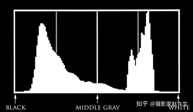
就是灰度级的统计图,横向是灰度级,纵向是出现的次数。
1.1 一般直方图
实现
I = imread('pout.tif');      %读取图像
figure;                      %打开一个窗口
imshow(I);title('Source');   %显示源图像
figure;                      %打开另一个窗口
imhist(I);title('Histogram');%显示直方图
1.2 归一化直方图
为便于统计,可根据区间统计灰度级,进行归一化。
实现
I = imread('pout.tif');
figure;
[M,N] = size(I);            %计算图像大小
[counts,x] = imhist(I,32);  %先计算32个小区间的灰度直方图
counts = counts /M / N;     %计算归一化灰度直方图各区间的值
stem(x,counts);             %绘制归一化直方图
1.3 应用
图像的灰度直方图有很多信息,如亮度和对比度等
亮度:灰度级集中位置,从左到右,图像逐渐变亮。
对比度:灰度级分布的区间越大,对比度越高。
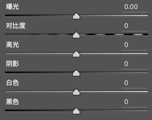
2 灰度的线性变换
利用一个一维线性函数实现对比度、亮度的变化:
S = f(t) = At + B。
其中,A对应对比度,A>1时,对比度增大;A B对应亮度,在A=1的条件下,B越大灰度值越大;A
实现
I = imread('coins.png');		% 读入原图像I = im2double(I);			% 转换数据类型为double
[M,N] = size(I);			% 计算图像面积figure(1);				% 打开新窗口
imshow(I);				% 显示原图像
title('原图像');figure(2);				% 打开新窗口
[H,x] = imhist(I, 64);		% 计算64个小区间的灰度直方图
stem(x, (H/M/N), '.');		% 显示原图像的直方图
title('原图像');% 增加对比度
Fa = 2; Fb = -55;
O = Fa .* I + Fb/255;figure(3);
subplot(2,2,1);
imshow(O);
title('Fa = 2 Fb = -55 增加对比度');figure(4);
subplot(2,2,1);
[H,x] = imhist(O, 64);
stem(x, (H/M/N), '.');
title('Fa = 2 Fb = -55 增加对比度');% 减小对比度
Fa = 0.5; Fb = -55;
O = Fa .* I + Fb/255;figure(3);
subplot(2,2,2);
imshow(O);
title('Fa = 0.5 Fb = -55 减小对比度');figure(4);
subplot(2,2,2);
[H,x] = imhist(O, 64);
stem(x, (H/M/N), '.');
title('Fa = 0.5 Fb = -55 减小对比度');% 线性增加亮度
Fa = 1; Fb = 55;
O = Fa .* I + Fb/255;figure(3);
subplot(2,2,3);
imshow(O);
title('Fa = 1 Fb = 55 线性平移增加亮度');figure(4);
subplot(2,2,3);
[H,x] = imhist(O, 64);
stem(x, (H/M/N), '.');
title('Fa = 1 Fb = 55 线性平移增加亮度');% 反相显示
Fa = -1; Fb = 255;
O = Fa .* I + Fb/255;figure(3);
subplot(2,2,4);
imshow(O);
title('Fa = -1 Fb = 255 反相显示');figure(4);
subplot(2,2,4);
[H,x] = imhist(O, 64);
stem(x, (H/M/N), '.');
title('Fa = -1 Fb = 255 反相显示');
3 灰度对数变换
这是一种灰度的非线性变换,可以增强较暗的区域:
t = c log(1+s)
实现
I = imread('coins.png');
F = fft2(im2double(I));%快速傅里叶变换计算频谱
F = fftshift(F);%将零频分量移到频谱中心
F = abs(F);%取正值
T = log(F + 1);%对数变换subplot(1,2,1);
imshow(F,[]);
title('对数变换前');subplot(1,2,2);
imshow(T,[]);
title('对数变换后');
4 伽玛变换
这是另一种常用的灰度非线性变换,用于增强对比度:
y = (x + esp)*r
式中,x与y的取值范围均为[0,1];esp为补偿系数;r为伽玛系数。
r>1时,图像的高灰度区域对比度增强。
实现
I = imread('pout.tif');subplot(1,3,1);
imshow(imadjust(I, [ ], [ ], 0.75));% Gamma取0.75
title('Gamma 0.75');subplot(1,3,2);
imshow(imadjust(I, [ ], [ ], 1));% Gamma取1
title('Gamma 1');subplot(1,3,3);
imshow(imadjust(I, [ ], [ ], 1.5));% Gamma取1.5
title('Gamma 1.5');figure;subplot(1,3,1);
imhist(imadjust(I, [ ], [ ], 0.75));% Gamma取0.75
title('Gamma 0.75');subplot(1,3,2);
imhist(imadjust(I, [ ], [ ], 1));% Gamma取1
title('Gamma 1');subplot(1,3,3);
imhist(imadjust(I, [ ], [ ], 1.5));% Gamma取1.5
title('Gamma 1.5');
5 灰度阈值变换
简单来说就是设置一个阈值,把灰度图变成二值图,小于阈值的就置0,大于阈值的置1。
实现
I = imread('rice.png');
thresh = graythresh(I);
bw1 = im2bw(I,thresh);
bw2 = im2bw(I,130/255);
subplot(1,3,1);imshow(I);title('原图像');
subplot(1,3,2);imshow(bw1);title('自动选择阈值');
subplot(1,3,3);imshow(bw2);title('阈值130');
6 分段线性变换
就是分段去增强或抑制灰度区域。
实现
首先自定义函数.m
function out = imgrayscaling(varargin)
% IMGRAYSCALING     执行灰度拉伸功能
%   语法:
%       out = imgrayscaling(I, [x1,x2], [y1,y2]);
%       out = imgrayscaling(X, map, [x1,x2], [y1,y2]);
%       out = imgrayscaling(RGB, [x1,x2], [y1,y2]);
%   这个函数提供灰度拉伸功能,输入图像应当是灰度图像,但如果提供的不是灰度
%   图像的话,函数会自动将图像转化为灰度形式。x1,x2,y1,y2应当使用双精度
%   类型存储,图像矩阵可以使用任何MATLAB支持的类型存储。[A, map, x1 , x2, y1, y2] = parse_inputs(varargin{:});% 计算输入图像A中数据类型对应的取值范围
range = getrangefromclass(A);
range = range(2);% 如果输入图像不是灰度图,则需要执行转换
if ndims(A)==3,% A矩阵为3维,RGB图像A = rgb2gray(A);
elseif ~isempty(map),% MAP变量为非空,索引图像A = ind2gray(A,map);
end % 对灰度图像则不需要转换% 读取原始图像的大小并初始化输出图像
[M,N] = size(A);
I = im2double(A);		% 将输入图像转换为双精度类型
out = zeros(M,N);% 主体部分,双级嵌套循环和选择结构
for i=1:Mfor j=1:Nif I(i,j)x2out(i,j) = (I(i,j)-x2)*(range-y2)/(range-x2) + y2;elseout(i,j) = (I(i,j)-x1)*(y2-y1)/(x2-x1) + y1;endend
end% 将输出图像的格式转化为与输入图像相同
if isa(A, 'uint8') % uint8out = im2uint8(out);
elseif isa(A, 'uint16')out = im2uint16(out);
% 其它情况,输出双精度类型的图像
end% 输出:
if nargout==0 % 如果没有提供参数接受返回值imshow(out);return;
end
%-----------------------------------------------------------------------------
function [A, map, x1, x2, y1, y2] = parse_inputs(varargin);
% 这就是用来分析输入参数个数和有效性的函数parse_inputs
% A       输入图像,RGB图 (3D), 灰度图 (2D), 或者索引图 (X)
% map     索引图调色板 (:,3)
% [x1,x2] 参数组 1,曲线中两个转折点的横坐标
% [y1,y2] 参数组 2,曲线中两个转折点的纵坐标
% 首先建立一个空的map变量,以免后面调用isempty(map)时出错
map = [];%   IPTCHECKNARGIN(LOW,HIGH,NUM_INPUTS,FUNC_NAME) 检查输入参数的个数是否
%   符合要求,即NUM_INPUTS中包含的输入变量个数是否在LOW和HIGH所指定的范围
%   内。如果不在范围内,则此函数给出一个格式化的错误信息。
iptchecknargin(3,4,nargin,mfilename);%   IPTCHECKINPUT(A,CLASSES,ATTRIBUTES,FUNC_NAME,VAR_NAME, ARG_POS) 检查给定
%   矩阵A中的元素是否属于给定的类型列表。如果存在元素不属于给定的类型,则给出
%   一个格式化的错误信息。
iptcheckinput(varargin{1},...{'uint8','uint16','int16','double'}, ...{'real', 'nonsparse'},mfilename,'I, X or RGB',1);switch nargincase 3 %            可能是imgrayscaling(I, [x1,x2], [y1,y2]) 或 imgrayscaling(RGB, [x1,x2], [y1,y2])A = varargin{1};x1 = varargin{2}(1);x2 = varargin{2}(2);y1 = varargin{3}(1);y2 = varargin{3}(2);case 4A = varargin{1};%               imgrayscaling(X, map, [x1,x2], [y1,y2])map = varargin{2};x1 = varargin{2}(1);x2 = varargin{2}(2);y1 = varargin{3}(1);y2 = varargin{3}(2);
end% 检测输入参数的有效性
% 检查RGB数组
if (ndims(A)==3) && (size(A,3)~=3)   msg = sprintf('%s: 真彩色图像应当使用一个M-N-3维度的数组', ...upper(mfilename));eid = sprintf('Images:%s:trueColorRgbImageMustBeMbyNby3',mfilename);error(eid,'%s',msg);
endif ~isempty(map)
% 检查调色板if (size(map,2) ~= 3) || ndims(map)>2msg1 = sprintf('%s: 输入的调色板应当是一个矩阵', ...upper(mfilename));msg2 = '并拥有三列';eid = sprintf('Images:%s:inColormapMustBe2Dwith3Cols',mfilename);error(eid,'%s %s',msg1,msg2);elseif (min(map(:))<0) || (max(map(:))>1)msg1 = sprintf('%s: 调色板中各个分量的强度 ',upper(mfilename));msg2 = '应当在0和1之间';eid = sprintf('Images:%s:colormapValsMustBe0to1',mfilename);error(eid,'%s %s',msg1,msg2);end
end% 将int16类型的矩阵转换成uint16类型
if isa(A,'int16')A = int16touint16(A);
end
调用代码
I = imread('coins.png');
J1 = imgrayscaling(I,[0.3 0.7],[0.15 0.85]);
J2 = imgrayscaling(I,[0.15 0.85],[0.3 0.7]);subplot(1,2,1);
imshow(J1,[]);subplot(1,2,2)
imshow(J2,[]);
7 直方图均衡化
简单的说就是,把灰度级近似均匀分布在各个像素上。
中的函数可自动实现该功能。
实现
I = imread('pout.tif');
I = im2double(I);% 对于对比度变大的图像
I1 = 2 * I - 55/255;
subplot(4,4,1);
imshow(I1);
subplot(4,4,2);
imhist(I1);
subplot(4,4,3);
imshow(histeq(I1));
subplot(4,4,4);
imhist(histeq(I1));% 对于对比度变小的图像
I2 = 0.5 * I + 55/255;
subplot(4,4,5);
imshow(I2);
subplot(4,4,6);
imhist(I2);
subplot(4,4,7);
imshow(histeq(I2));
subplot(4,4,8);
imhist(histeq(I2));% 对于线性增加亮度的图像
I3 = I + 55/255;
subplot(4,4,9);
imshow(I3);
subplot(4,4,10);
imhist(I3);
subplot(4,4,11);
imshow(histeq(I3));
subplot(4,4,12);
imhist(histeq(I3));% 对于线性减小亮度的图像
I4 = I - 55/255;
subplot(4,4,13);
imshow(I4);
subplot(4,4,14);
imhist(I4);
subplot(4,4,15);
imshow(histeq(I4));
subplot(4,4,16);
imhist(histeq(I4));
8 直方图规定化
有时需要某种特定的直方图的形状,那么就要有选择地增强或者特定分布等操作了。
实现
I = imread('pout.tif'); %读入原图像
I1 = imread('coins.png'); %读入要匹配直方图的图像
I2 = imread('circuit.tif'); %读入要匹配直方图的图像% 计算直方图
[hgram1, x] = imhist(I1);
[hgram2, x] = imhist(I2);% 执行直方图均衡化
J1=histeq(I,hgram1);
J2=histeq(I,hgram2);% 绘图
subplot(2,3,1);
imshow(I);title('原图');
subplot(2,3,2);
imshow(I1); title('标准图1');
subplot(2,3,3);
imshow(I2); title('标准图2');
subplot(2,3,5);
imshow(J1); title('规定化到1')
subplot(2,3,6);
imshow(J2);title('规定化到2');% 绘直方图
figure;subplot(2,3,1);
imhist(I);title('原图');subplot(2,3,2);
imhist(I1); title('标准图1');subplot(2,3,3);
imhist(I2); title('标准图2');subplot(2,3,5);
imhist(J1); title('规定化到1')subplot(2,3,6);
imhist(J2);title('规定化到2');