related Alignment for Universal Zero

论文地址：

项目主页：

代码：

We study zero-shot in this work to , , and for novel any 。 Such zero-shot on inter-class in space to the from seen to ones。 Thus, it is to well - and apply the to 。 We a model to for , which links and as well as the issue of lack of data。

, to the gap and , , we the with , each of which fine- to , and by these 。 , we to the into the - part and the - part that clues but is less to 。

The inter-class of - are then to be with those in space, to 。 The state-of- on zero-shot , , and 。

本文研究了通用的零样本分割，在不需要任何训练样本的情况下，实现新类别的全景、实例和语义分割。这种零样本分割能力依赖于语义空间中的类间关系，将从可见类别中学习到的视觉知识转移到不可见类别中。因此，希望很好地桥接语义视觉空间，并将语义关系应用于视觉特征学习。我们引入了一个生成模型来合成不可见类别的特征，该模型连接了语义和视觉空间，并解决了缺乏不可见训练数据的问题。此外，为了缓解语义空间和视觉空间之间的领域差距，首先，我们用学习基元增强经典生成器，每个基元都包含与类别相关的细粒度属性，并通过选择性地组装这些基元来合成看不见的特征。其次，我们建议将视觉特征分为语义相关部分和语义无关部分，语义相关部分包含有用的视觉分类线索，但与语义表示不太相关。然后，与语义相关的视觉特征的类间关系需要与语义空间中的那些类间关系对齐，从而将语义知识转移到视觉特征学习中。该方法在零样本全景分割、实例分割和语义分割方面取得了令人印象深刻的性能。

1.

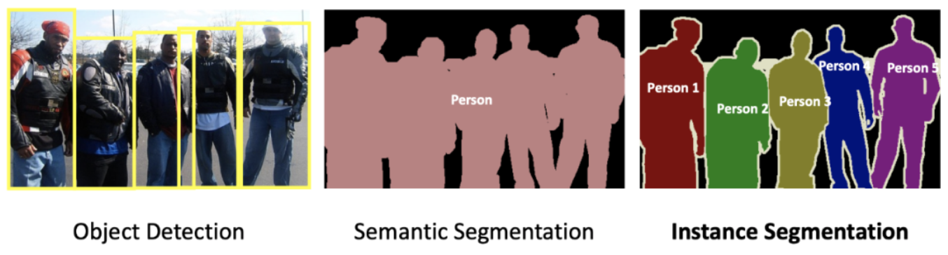
Image aims to group with , e.g., or [11,41]. Deep [9, 11, 17, 29, 36, 37, 48] have the of image with the of CNNs [30] and [59]. , since deep are data-, are by the for , which are labor- and time-. To this issue, zero-shot (ZSL) [38,51] is to novel with no . , ZSL is into tasks like zero-shot (ZSS) [4, 62] and zero-shot (ZSI) [68]. , we zero-shot (ZSP) and aim to build a for zero-shot // with the help of , as shown in Fig. 1.

图像分割旨在对具有不同语义的像素进行分组，例如类别或实例[11，41]。深度学习方法[9，11，17，29，36，37，48]凭借CNN[30]和[59]强大的学习能力，极大地提高了图像分割的性能。然而，由于深度学习方法是数据驱动的，对大规模标记训练样本的强烈需求带来了巨大的挑战，这是劳动密集型和耗时的。为了解决这个问题，提出了零样本学习（ZSL）[38,51]来对没有训练样本的新对象进行分类。最近，ZSL被扩展为零样本语义分割（ZSS）[4，62]和零样本实例分割（ZSI）[68]等分割任务。在此，我们进一步介绍了零样本全景分割（ZSP），旨在借助语义知识构建一个通用的零样本全景/语义/实例分割框架，如图1所示。

1. Zero-shot image aims to the from seen to ones (i.e., never shown up in ) with the help of

图1。零样本图像分割的目的是借助语义知识将从可见类中学习到的知识转移到不可见类（即从未在训练中出现）

from image , pixel-wise and is more in terms of class . have been to zero-shot [4, 62] and can be into -based [20, 62, 66] and model-based [4, 27, 40]. The model-based are to the -based they for the group, which to the bias issue [53] of to into seen . Owing to the above , we the of model-based to zero-shot tasks.

与图像分类不同，分割需要逐像素分类，并且在类表示学习方面更具挑战性。零样本语义分割[4，62]已经投入了大量的努力，可以分为基于投影的方法[20，62，66]和基于生成模型的方法[4，27，40]。基于生成模型的方法通常优于基于投影的方法，因为它们为看不见的组生成合成训练特征，这有助于缓解倾向于将对象分类为可见类的关键偏差问题[53]。由于上述优点，我们遵循基于生成模型的方法的范式来处理零样本分割任务。

, the model-based are in the form of per-pixel-level , which is not in the more 。 , works to the into class- mask and -level [8, 11, 31, 61]。 We this and the pixel-level to a more -level 。 What’s more, works [4, 27, 40] learn a from to 。

Such a does not the - gap of that much than 。 The from to in low- 。 To this issue, we to with very fine- to 。 of these class , where the is by the and 。

the and of the , in terms of rich fine- , the for more and 。

然而，目前基于生成模型的方法通常是以每像素级生成的形式，在更复杂的场景中不够鲁棒。最近，一些工作提出将分割解耦为类不可知的掩码预测和对象级分类[8，11，31，61]。我们遵循这一策略，并将像素级生成退化为更稳健的对象级生成。此外，以前的生成作品[4，27，40]通常学习从语义嵌入到视觉特征的直接映射。这样的生成器没有考虑特征粒度的视觉语义差距，即图像包含比语言丰富得多的信息。从粗信息到细粒度信息的直接映射导致低质量的合成特征。为了解决这个问题，我们提出利用具有非常细粒度语义属性的丰富来组成视觉表示。这些的不同集合构造不同的类表示，其中集合由基元和语义嵌入之间的相关性决定。极大地增强了生成器的表达多样性和有效性，特别是在丰富的细粒度属性方面，使不同类别的合成特征更加可靠和具有鉴别性。

, there are only real image of seen to the , 。 To more for the of , we to the inter-class in space to space。 The by are to the inter-class of 。 With such , the , the for , are to have a inter-class as in space。

, there is a the space and the space [10, 57], so as to their inter-class 。 and be fully with 。 two the of 。 To this issue, we to into - and , where the is with the while the is noisy to space。

We only use - for 。 The and are 。 - space to and that are noisy for 。 in turn to by clues。

然而，只有可见类的真实图像特征来监督生成器，而不监督不可见类。为了给看不见类的特征生成提供更多的约束，我们建议将语义空间中的类间关系转移到视觉空间。通过语义嵌入获得的类别关系用于约束视觉特征的类间关系。在这样的约束下，视觉特征，特别是看不见类的合成特征，被提升为在语义空间中具有同构的类间结构。然而，视觉空间和语义空间之间存在差异[10，57]，因此它们的类间关系也存在差异。视觉特征包含更丰富的信息，不能与语义嵌入完全一致。直接对齐两个不相交的关系不可避免地会损害视觉特征的辨别力。为了解决这个问题，我们建议将视觉特征分为语义相关和语义无关特征，其中前者与语义嵌入更好地对齐，而后者对语义空间有噪声。我们只使用语义相关的特征来进行关系对齐。所提出的关系对齐和特征解纠缠是互利的。特征解纠缠建立了语义相关的视觉空间，以促进关系对齐，并排除了对对齐有噪声的语义无关特征。关系对齐反过来又通过提供语义线索来帮助解开语义相关的特征。

, the main are as :总体而言，主要贡献如下：

• We study zero-shot and with and () as a for ZSP/ZSI/ZSS.•我们研究了通用零样本分割，并提出了使用协作关系对齐和特征去纠缠学习（）的原语生成，作为ZSP/ZSI/ZSS的统一框架。

• We a that lots of with fine- to for , which helps to the bias issue and gap issue.•我们提出了一种基元生成器，该生成器使用大量具有细粒度属性的学习基元来合成看不见类别的视觉特征，这有助于解决偏差问题和领域差距问题。

• We a and to the .•我们提出了一种协作关系对齐和特征解纠缠学习方法，以促进生成器生成更好的合成特征。

• The new -the-art on zero-shot (ZSP), zero-shot (ZSI), and zero-shot (ZSS).•所提出的方法在零样本全景分割（ZSP）、零样本实例分割（ZSI）和零样本语义分割（ZSS）方面实现了最新的性能。

2. Work

Zero-shot (ZSL) [35, 38, 51, 67] aims to of with no via as . There are two main : -based that learn a - [1, 42, 67] and -based [21, 64] that fake for . zero-shot (GZSL), by et al. [55], aims to from both seen and sets. Then, Chao et al. [6] show that the ZSL can’t work well in GZSL from , due to the of on seen . score [5,13, 28, 33] and out-of- [3, 24] are to this bias issue.

零样本学习（ZSL）[35，38，51，67]旨在利用语义描述符作为辅助信息，对没有训练样本的未见过类的图像进行分类。有两种主要的范式：学习视觉语义投影的基于分类器的方法[1，42，67]和为看不见的类合成假样本的基于实例的方法[21，64]。广义零样本学习（GZSL）由等人[55]引入，旨在对可见和不可见集合中的样本进行分类。然后，Chao等人[6]从实验中表明，ZSL方法在GZSL设置中不能很好地工作，这是由于对可见类的过拟合特性。提出了分类分数校准方法[5，13，28，33]和分布外检测器方法[3，24]来缓解这种偏差问题。

Image is one of the most tasks [14,18,19,22,45,46]。 Deep- image under a fully are [9, 11, 15, 16, 29, 36, 37, 47, 48, 56, 61]。 , these a large of and that do not or are not in data。 To these , Zero-Shot (ZSS) [4] and Zero-Shot (ZSI) [68] ZSL to and , 。

In this work, we Zero-Shot (ZSP) to the zero-shot to the task。 There are two main : -based [8, 20, 32, 49, 52, 62, 63, 66] and -based [4, 12, 40]。 -based a to map the or of seen onto a space。 (e。g。, , , or space), and then novel by the in the space。

The adopt to for 。 , works [4, 27, 40] learn a from to and do not the - gap of 。 We a and - to zero-shot , ZSP, ZSI, and ZSS。

图像分割是最基本的计算机视觉任务之一[14，18，19，22，45，46]。广泛研究了完全监督方式下基于深度学习的图像分割方法[9，11，15，16，29，36，37，47，48，56，61]。然而，这些方法需要大量标记的训练样本，并且不能处理在训练数据中没有出现或没有定义的看不见的类别。为了解决这些问题，零样本语义分割（ZSS）[4]和零样本实例分割（ZSI）[68]分别将ZSL方法扩展到语义分割和实例分割。在这项工作中，我们进一步引入了零样本全景分割（ZSP），将零样本学习扩展到全景分割任务中。有两种主要的范式：基于投影的方法[8，20，32，49，52，62，63，66]和基于生成的方法[4，12，40]。基于投影的技术通常利用投影方法将所看到的类别的视觉或语义特征映射到共享空间上。（例如，视觉、语义或潜在空间），然后通过测量公共空间中的特征相似性来对新对象进行分类。生成方法采用生成器为看不见的类生成合成特征。然而，现有的生成工作[4，27，40]通常学习从语义嵌入到视觉特征的直接映射，并且没有考虑特征粒度的视觉语义差距。我们设计了一种原语生成和语义相关的对齐方法来通用地处理零样本分割，包括ZSP、ZSI和ZSS。

3.

Fig. 2 the of our , with and (). Our a set of class- masks and their class . is to class from . The real & class are to - and - . We the on the - . With the class , we re-train our with both the real class of seen and the class of . The is in 1. The of each part will be in the .

图2说明了我们提出的方法的总体架构，具有协作关系对齐和特征去纠缠学习（）的原始生成。我们的主干预测了一组类不可知掩码及其相应的类嵌入。基元生成器被训练为从语义嵌入中合成类嵌入。真实的和合成的类嵌入被分解为语义相关和语义无关的特征。我们对语义相关特征进行关系对齐学习。使用合成的不可见类嵌入，我们用可见类别的真实类嵌入和不可见类别的合成类嵌入来重新训练我们的分类器。训练过程在算法1中进行了演示。每个部分的细节将在以下章节中介绍。

2. of our for zero-shot image . We first class- masks and their , named class , from our . A is to (i.e., fake class ). The , which takes class as input, is with both the real class from image and class by the . the of the , the and are to the .

图2:概述我们用于通用零样本图像分割的方法。我们首先从主干中获得类不可知掩码及其相应的全局表示，即命名的类嵌入。原始生成器被训练来产生合成特征（即，假类嵌入）。分类器以类嵌入作为输入，由生成器使用来自图像的真实类嵌入和合成类嵌入来训练分类器。在生成器的训练过程中，采用所提出的特征解纠缠和关系对齐来约束合成的特征。

3.1. Task

we give the of zero-shot image 。 There are two , space X and space A, to the of and of , as X = {Xs , Xu}, A = {As , Au}, 。 The s and u the two non- , Ns seen and Nu ,。 We use Y = {Y s , Y u} to the truth label。 Y s is label set of seen group and Y u is label set of group, Y s ∩ Y u = ∅。

The set is from the that any of the Ns seen but no , which is from the open- [34, 65]。 to the that in the set, there are two named zero-shot (ZSL) and zero-shot (GZSL)。 ZSL only of while GZSL needs to data of both seen and 。 Zero-shot is a kind of GZSL since the and 。 In this work, all the zero-shot tasks are under the GZSL 。

这里我们给出了零样本图像分割的问题公式。有两个空间，特征空间X和语义空间A，分别表示图像的视觉特征和类别的语义表示，表示为X={Xs，Xu}，A={as，Au}。上标s和u分别表示两个不重叠的组，即Ns可见类别和Nu不可见类别。我们使用Y={Ys，Yu}来表示地面实况标签。Y s是可见群的标签集，Y u是不可见群的标记集，Y s≠Y u=∅。训练集是由包含任何Ns个可见类别但没有未可见类别的图像构建的，这与开放词汇范式（ open- ）不同[34，65]。根据测试集中出现的类别，有两种不同的设置，称为零样本学习（ZSL）和广义零样本学习（GZSL。ZSL只对看不见类别的测试样本进行分类，GZSL需要对看不到类别的测试数据进行分类。零样本分割自然是一种GZSL，因为图像通常包含多种多样的类别。在本工作中，除非另有规定，否则所有零样本分割任务都在GZSL设置下。

3.2. Cross-Modal

Due to the lack of , the be with of 。 As a , the on seen tends to all /stuff a label of seen group, which is bias issue [6]。 To this issue, [4,27,40] to a model to fake for 。 , zero-shot works [4, 27, 40] adopt (GMMN) [40,43] or GAN [25], which of as 。

Such a , good , does not the - of 。 It is well known that image much than 。 very fine- of while and high-level 。 Such in an in- and 。 To this , we a that lots of to 。

由于缺乏看不见的样本，分类器无法使用看不见类的特征进行优化。因此，在可见类上训练的分类器倾向于为所有对象/材料分配可见组的标签，这被称为偏差问题[6]。为了解决这个问题，以前的方法[4，27，40]提出利用生成模型来合成看不见类的虚假视觉特征。然而，以往的生成性零样本分割工作[4、27、40]通常采用生成性矩匹配网络（ ，GMMN）[40、43]或GAN[25]，它们由多个线性层组成，作为特征生成器。这样的生成器虽然取得了良好的性能，但没有考虑特征粒度的视觉语义差异。众所周知，图像通常比语言包含更丰富的信息。视觉信息提供对象的细粒度属性，而文本信息通常提供抽象和高级属性。这种差异导致视觉特征和语义特征之间的一致性。为了解决这一挑战，我们提出了一种基元交叉模态生成器，该生成器使用大量学习的属性基元来构建视觉表示。

[4] , Tuan-Hung Vu, Cord, and Perez. Zero-shot . ´ , 32, 2019. 1, 2, 3, 4, 6, 8

[27] Gu, Zhou, Li Niu, Zihan Zhao, and Zhang. -aware for . In ACM MM, 2020. 1, 2, 3, 4, 8

[40] Peike Li, Wei, and Yi Yang. for zero-shot . , 33, 2020. 1, 2, 3, 4

As shown in Fig. 3, we build our with a . First, a set of are , as P = {pi} N i=1, where pi ∈ R dk and dk is the of . These are to very fine- to , e.g., hair, color, shape, etc. kinds of of these build for . A self- is first on these to graph among these . Next, we two ωK and ωV to deal with P to the Key and Value for cross , as K and V . Then, as Query Q, cross is as

如图3所示，我们使用架构构建了 。首先，随机初始化一组可学习基元，表示为P={pi}NI=1，其中pi∈Rdk，dk是通道数。假设这些基元包含与类别相关的非常细粒度的属性，例如头发、颜色、形状等。这些基元的不同类型的组合为类别构建了不同的表示。首先对这些基元进行自关注，构建这些基元之间的关系图。接下来，我们利用两个不同的线性层ωK和ωV来处理P，以获得交叉注意的密钥和值，分别表示为K和V。然后，将语义嵌入作为查询Q，执行交叉注意如下

where X ′ and Z with a fixed . ω1 is the layer. from via with , we via these , which much more and . , for that share some in space, an way to such . For , dog and cat both have the of hairy and tail, so the to hairy and tail show high to the query of dog and cat. With such that fine- , we can and the of seen to ones.

其中X′表示合成视觉特征，Z表示具有固定高斯分布的随机样本。ω1是线性层。与通过处理具有多个线性层的语义嵌入来生成特征不同，我们通过加权组装这些丰富的基元来合成视觉特征，这提供了更多样、更丰富的表示。此外，对于在语义空间中具有某些相似性的相关类别，原语提供了一种明确的方式来表达这些相似性。例如，dog和cat都具有毛和尾巴的属性，因此与毛和尾巴相关的原语对dog和cat的语义嵌入查询显示出较高的响应。有了这些描述细粒度属性的原语，我们可以很容易地构建不同的类别表示，并将可见类的知识转移到不可见类。

We [43] to our loss LG to mean two :

我们按照[43]定义我们的生成器损失LG，以减少两个概率分布之间的最大平均差异：

where Xs and Xs′ real and of seen , . k is a and k(f, f′ ) = exp(− 1 2σ2 ∥f − f ′∥ 2 ) with σ

其中Xs和Xs′分别表示可见类的真实视觉特征和合成视觉特征。k是一个核，k（f，f′）=exp（−12σ2½f−f′½2），带宽为σ

When a from group is fed into the , we can get its class . We then re-train our with both the real class of seen and the class of , which the bias issue. , such are more than per-pixel [4, 27, 40, 66, 68] and can thus have a space and space.

当一个来自看不见组的语义嵌入被输入到训练过的原始生成器中时，我们可以得到它相应的合成类嵌入。然后，我们用可见类别的真实类嵌入和不可见类别的合成类嵌入来重新训练我们的分类器，这大大缓解了偏差问题。此外，这种全局表示比每像素分类[4，27，40，66，68]更稳健，因此可以在视觉空间和语义空间之间具有更好的一致性。

3.3. -

It is well known that among are [7, 40, 60]. For , there are three : apple, , and cow. , the of apple & is than apple & cow. Class in space are prior , while the does not such . As shown in Fig. 4, we build such with and to this to space, in terms of class-wise . By the , there are more on the ’ , to pull or push their with seen .

众所周知，类别之间的关系自然是不同的[7，40，60]。例如，有三个对象：苹果、桔子和奶牛。显然，苹果和桔子的关系比苹果和奶牛的关系更密切。语义空间中的类关系是强大的先验知识，而特定于类别的特征生成并没有明确地利用这些关系。如图4所示，我们用语义嵌入建立了这样的关系，并探索将这些知识转移到视觉空间，根据类关系进行语义视觉对齐。通过考虑这种关系，对看不见的类别的特征生成有更多的限制，以拉或推他们与看到的类别的距离。

4. . (a) The . (b) Our two-step . the gap, we a - space, where are from space and have more with space. We have the in - space be with space. ui/sj to /seen . u1 dog as an , we aim to its with {cat, , horse, zebra} from to space.

图4。关系调整。（a） 传统的关系调整。（b） 我们提出的两步关系调整。考虑到领域差距，我们引入了一个与语义相关的视觉空间，其中特征与视觉空间分离，与语义空间具有更直接的相关性。我们使语义相关的视觉空间中的关系与语义空间保持一致。ui/sj是指看不见/看到的类别。以u1狗为例，我们旨在将其与{猫、大象、马、斑马}的相似性从语义转移到视觉空间。

- , the are not fully with the but and also - 。 - may have clues and to , but have low with 。 with would the and its to 。

To this issue, we to the - and 。 Given a xi , where xi ∈ X is the class from or our , how to and xi 。 We use ER to - , xˆi = ER(xi)。 Then, we the score - xˆi and A = {a1, 。。。, aNs+Nu }。 ER is with cross- loss as a to endow - xˆi with , i。e。,

语义相关的视觉特征 然而，视觉特征并不完全与语义表示一致，而是包含更丰富的信息，包括语义相关的可视特征和语义无关的可视特征。语义无关特征可能具有较强的视觉线索，有助于分类，但与语言语义表示的相关性较低。直接将语义嵌入与原始视觉特征对齐会混淆生成器，并减少其对看不见的类别的泛化。为了解决这个问题，我们建议将语义相关的视觉特征和语义无关的视觉特征区分开来。给定一个特征xi，其中xi∈X是从主干或生成器嵌入的类，特征解缠结学习如何解缠结和重建xi本身。我们使用编码器ER提取语义相关特征，xˆi=ER（xi）。然后，我们计算语义相关特征xõi和语义嵌入A={a1，…，aNs+Nu}之间的相关性得分。ER是用交叉熵损失作为分类问题来训练的，以赋予语义相关特征xõi判别语义知识，即。，

where [ˆxi ] is the truth class intex of xˆi , 1(·) is the that 1 if the is true and 0 . τ is the .

其中[ˆxi]是x \710»i的基本真值类intex，1（·）是指示函数，如果条件为真，则输出1，否则输出0。τ是温度参数。

We use EU to , as x¨i = EU(xi). We the - to have the N (0, 1) with zero mean and unit [39]. We use KL loss to the range,

我们使用另一个编码器EU提取与语义相关的特征，表示为x¨i=EU（xi）。我们假设语义无关的特征具有正态分布N（0，1），平均值和单位方差为零[39]。我们使用KL发散损失来约束分布范围，

where DKL[p||q] = − R p(z)log p(z) q(z) . Such that each class has its own and . To push the to more and , we the with a D under ℓ1 loss:

式中DKL[p||q]=−R p（z）log p（z）q（z）。使得每个类都有自己独立和多样化的特征组件。为了推动网络提取更具代表性的语义相关特征并保存视觉特征信息，我们在解码器中引入ℓ1损失：

The for is LD = LR + LU + .

特征解纠缠的训练目标是LD=LR+LU+。

Then we - space and space. We use KL loss to make the of any two - xˆi and xˆj reach the of their a[ˆxi] and a[ˆxj ] , i.e.,

关系对齐 然后我们在语义相关的视觉空间和语义空间之间进行关系对齐。我们使用KL散度损失使任何两个语义相关特征xˆi和xᮼj的相似性达到其对应语义嵌入a[\710,xi]和a[ڮxj]的相似性，即：

where [ˆxi ] is the truth class index of xˆi , τ is the to the of on the KL loss。 xˆ s i of the seen group is from real or while xˆ u i of the group is from by only。 There are two kinds of , and inter-group , with in Eq。 (6)。 When xˆi and xˆj are from the same group, e。g。, xˆ s i and xˆ s j both from seen group, it is and to class with the as a 。

When they are from , e。g。, xˆ s i from seen group and xˆ u j from group, it is inter-group that aims to the from seen to 。 Inter-group gives on the of seen and , real and 。 It the model’s and to 。

其中[ˆxi]是x \710»i的基本真值类指数，τ是控制KL损失上相似分布清晰度的温度参数。看到的组的xŞs i来自真实特征或合成特征，而看不见的组的xŞu i仅来自生成器的合成特征。有两种对齐，组内对齐和组间对齐，在等式中焦点不同。（6）。当x Plot i和x Plot j来自同一组时，例如，x Plot s i和xës j都来自可见组，这是组内对齐，并有助于提取更好的类表示，其中关系作为约束。当它们来自不同的组时，例如，来自可见组的xŞs i和来自看不见组的xõu j，组间对齐旨在将关系知识从可见转移到看不见。组间对齐对可见和不可见类别、真实特征和合成特征之间的关系进行了约束。它大大提高了模型对不可见类别的适应性和泛化能力。

and Our and are and . On the one hand, . With the , - can be for and - are . On the other hand, . intra-group and inter-group , among - can be and the - can be , to the of the .

协同解纠缠与对齐 我们的解纠缠与对齐是相辅相成的。一方面，解开纠缠会促进关系的协调。通过解纠缠，可以提取与语义相关的特征进行对齐，并排除与语义无关的噪声。另一方面，关系对齐有助于解开纠缠。引入组内和组间对齐，可以构建语义相关特征之间的类关系，减少语义视觉特征分布之间的差异，最终改善特征解纠缠。

3.4.

1 shows the of our zero-shot model. First, we pre- with data from seen in a full- . Next, We train the under the :

算法1显示了通用零样本分割模型的整体训练流水线。首先，我们以完全监督的方式，用来自可见类的注释数据预训练我们的分割主干。接下来，我们在以下目标下训练原始生成器：

where λ is the to the of the and . Once the is above, it can for . with the real from seen , we can train a new layer.

其中λ是控制解纠缠和对准模块重要性的权重。一旦生成器在上面进行了训练，它就可以为看不见的类生成合成特征。结合可见类的真实特征，我们可以训练一个新的分类层。

4. 4.1. Setup

。 The and all our are based on 。 We CLIP text [54] and [50] as our and it with ℓ2 。 CLIP text are the works [20,26]。 We adopt [11] build upon the -50 as [30], with 100 for both and 。 Hyper- are with the of [11] 。 ER and EU are both multi-layer (MLP) one layer, and 。

ED is with two MLP by and 。 We apply SGD for the of with rate 1 × 10−3 , decay 5 × 10−4 and 0。9, and Adam for the of , ER, EU, and ED with rate 2 × 10−4 。 The of the , loss λ in Eq。 (7), τ , σ are set to 3, 0。002, 0。1, {2, 5, 10, 20, 40, 60}, 。

实施细节。所提出的网络和我们所有的实验都是基于实现的。我们使用CLIP文本嵌入[54]和[50]作为我们的语义嵌入，并用ℓ2标准化。CLIP文本嵌入是根据之前的工作[20，26]提取的。我们采用基于-50的[11]作为主干[30]，有100个查询用于训练和推理。除非另有规定，否则超参数与[11]的设置一致。编码器ER和EU都是多层感知器（MLP），包含一个隐藏层，激活和丢弃。ED由两个堆叠的单个MLP层构成，然后是激活和脱落。我们将SGD优化器应用于学习率为1×10−3、权重衰减为5×10−4和动量为0.9的分类器的参数，并将Adam优化器应用于生成器、ER、EU和ED的参数，初始学习率为2×10−4。变压器层数、等式中的损耗λ。（7）、温度τ、σ分别设置为3、0.002、0.1、{2、5、10、20、40、60}。

. We use the 2017, which set with 118k and set with 5k . For , 133 (80 thing and 53 stuff ) are in . For , COCO-Stuff 171 valid in total. To get a fair with ZSI [68], we use 2014 for which 80k and 40k .

数据集。我们使用流行的数据集 2017，该数据集由118k张图像的训练集和5k张图像的验证集组成。对于全景分割，注释中包括133个类（80个 thing 和53个stuff ）。对于语义分割，COCO Stuff总共包含171个有效类。为了与ZSI[68]进行公平的比较，我们使用 2014进行分割，该分割包含80k个训练图像和40k个验证图像。

4.2. Zero-Shot Task

of the high and , we the ZSP by the ZSS works [62]。 In order to avoid any , SPNet 15 in COCO stuff that do not in as 。 In COCO , we find 14 with the 15 ones by SPNet and set them as , i。e。, {cow, , , , , , , ,sky-other-, grass-, , river, road, tree-}, while the 119 are set as seen 。

To no in the set, we the that even one pixel of any 。 Thus the model is by of seen only with 45617 。 We use all 5k to the of ZSP。 and tasks are on the union of thing and stuff while is only on the thing 。

由于语义分割和全景分割之间的高度相似性，我们按照ZSS之前的工作开发了ZSP数据集[62]。为了避免任何信息泄露，SPNet在COCO中选择了15个没有出现在中的类作为不可见类。在COCO全景数据集中，我们发现14个类与SPNet选择的15个类重叠，并将它们设置为看不见的类，即{牛、长颈鹿、手提箱、飞盘、滑板、胡萝卜、剪刀、纸板、天空其他合并、草地合并、操场合并、河流合并、道路合并、树合并}，其余119个类设置为可见类。为了保证训练集中没有信息泄露，我们丢弃了包含任何看不见类的一个像素的训练图像。因此，该模型仅通过具有45617个训练图像的可见类的样本来训练。我们使用所有5k验证图像来评估ZSP的性能。泛光学和语义分割任务是在事物和事物类的并集上进行评估的，而实例分割仅在事物类上进行评估。

. Under the GZSL , the model needs to /stuff of both seen and , which is to real-world . ZSS [4, 62], ZSD [2], and ZSI [68] tasks, we seen , , and the mean (HM) of seen and as ,

评估指标。在GZSL设置下，模型需要分割可见类和不可见类的对象/东西，这更接近于现实世界中的复杂场景。在之前的ZSS[4，62]、ZSD[2]和ZSI[68]任务之后，我们计算可见度量、不可见度量以及可见度量和不可见度量的调和平均值（HM），如下所示，

where Pseen and the seen and , . We use the PQ ( ) [37] which can be as the of a (SQ) and a (RQ). We also the on , and tasks. For and , we use the mAP (mean ) [44] with an IoU of 0.5. For , we use mIoU (mean -over-Union) [23].

其中Pseen和分别表示可见和不可见度量。我们使用PQ（全景质量）度量[37]，它可以被视为分割质量（SQ）和识别质量（RQ）的乘积。我们还报告了实例分割、对象检测和语义分割任务的结果。例如，分割和对象检测，我们使用IoU阈值为0.5的标准mAP（平均平均精度）[44]。对于语义分割，我们使用mIoU（并集上的平均交集）[23]。

4.3. Study

In Tab。 1 and Tab。 2, We of the on MS-COCO under four tasks, zero-shot , zero-shot , zero-shot , and 。 It is worth that the in Tab。 2 are by the model on zero-shot task only, which our goal of a model for image tasks。 For , our on ZSP, ZSI, ZSD, ZSS have with ZSP。

First, to the of model, we a -based by using CLIP text as ’s , with -seg [20]。 , there are 119 text used in , while , we add 14 text into and label each to one of these 133 。 As the 2nd row in Tab。 1, there is a bias seen , in low even zero for group。

Next, we build upon GMMN model ZS3 [4], which n-based by 4。9% in terms of PQ。 This shows that model to bias issue。

在表1和表2中，我们在四个任务下对MS-COCO数据集上提出的进行消融研究，包括零样本全景分割、零样本实例分割、零样本对象检测和零快照语义分割。值得注意的是，表2中的结果是由仅针对零样本全景分割任务训练的模型获得的，这实现了我们为通用零快照图像分割任务训练单个模型的目标。为了简单起见，我们的烧蚀分析主要集中在ZSP上，因为ZSI、ZSD、ZSS与ZSP的趋势相似。首先，为了证明引入生成模型的优势，我们通过使用CLIP文本嵌入作为分类器的权重来实现基于投影的分割基线，类似于 seg[20]。在训练过程中，分类器中使用了119个文本嵌入，而在推理过程中，我们将另外14个看不见的文本嵌入添加到分类器中，并将每个对象标记到这133个类中的一个。如表1中的第二行所示，对可见类存在强烈的偏见，导致不可见组的精度极低，甚至为零。接下来，我们根据ZS3[4]在生成GMMN模型的基础上构建基线，该模型在看不见的PQ方面比基于投影的方法好4.9%。这一现象表明，生成模型有助于解决关键的偏差问题。

Table 1. Zero-shot study on . G, P, A, D GMMN , , , and , .

表1。上零样本全景分割消融研究结果。G、 P、A、D分别表示GMMN生成器、基元生成器、解纠缠和对准。

Table 2. study on ZSD, ZSI, and ZSS. G, P, A, D GMMN , , , and , . The our goal of a model for zero-shot image tasks.

表2。ZSD、ZSI和ZSS的烧蚀研究。G、 P、A、D分别表示GMMN生成器、基元生成器、解纠缠和对准。结果验证了我们为通用零样本图像分割任务训练单个模型的目标。

of . We the ’s with of in Tab. 3. From the , the from 100 to 400 a gain of 4.2%. The is a down when the is than 400, thus we 400 as the .

基本体的数量。我们在表3中报告了不同数量基元的网络性能。从结果来看，将基元数从100增加到400会带来4.2%的显著性能提升。当基元数大于400时，性能会略有下降，因此我们选择400作为默认设置。

of . Then, by as a to our , the HMPQ is by 2.6%, the of inter-class from space. , we the with , see 6) in Tab. 1 and Tab. 2. In to using only, + prior on - and gains of 2.0% HM-PQ, 13.3% HM-SQ, and 2.7% HM-RQ. The that the - has been owing to - . The of more in the - space.

调整的有效性。然后，通过将语义对齐作为约束应用于我们的生成器，HMPQ进一步提高了2.6%，证明了引入语义空间固有的类间关系的有效性。最后，我们评估了具有解纠缠的对齐模块，参见表1和表2中的6）。与仅使用对齐相比，对齐+解纠缠转移了语义相关特征的语义先验知识，并始终带来2.0%的HM-PQ、13.3%的HM-SQ和2.7%的HM-RQ的性能增益。显著的改进表明，由于省略了语义无关的噪声，语义视觉差异得到了缓解。解纠缠的利用使得能够在分离的语义相关空间中进行更有效的对齐。

of . To study the of our and the of our , we t-SNE [58] to show the of our in Fig. 5. As we can see in Fig. 5 (a), the by GMMN are messy due to the - . In Fig. 5 (b), when our , to the same class more and from are . , after - on the - , see Fig. 5 (c), to are apart with - , which shows that the is into and the are with .

合成特征表示的可视化。为了研究我们合成的看不见特征的性质并证明我们提出的方法的有效性，我们使用t-SNE[58]在图中显示了我们合成特征的分布。5。如图6所示，如图5（a）所示，由于语义-视觉差异，GMMN生成器生成的合成特征是混乱的。在图5（b）中，当引入我们的原始生成器时，属于同一类的特征变得更加紧凑，并且来自不同类的特征是高度可分离的。此外，在对语义相关特征应用关系对齐约束后，见图5（c），属于不同类别的特征之间的距离更远，具有更好的结构化分布，这表明结构关系嵌入了合成特征中，合成的不可见特征得到了更好的区分，大大增强。

4.4. with State-of-the-art ZSS

To the of our , we it with state-of-the-art ZSS on the in Tab. 4. It is worth that we only self- and crop-mask image for CLIP image for a . We train our model with . The the best -seg [20] by 3.5% HM-IoU and 3.4% -IoU, its . It is worth that the above use -101 while we only use -50.

为了进一步验证我们的方法的优越性，我们在表4中富有挑战性的语义分割数据集上将其与以前最先进的ZSS方法进行了比较。值得注意的是，我们只报告了没有自我训练的结果，也没有用于CLIP图像编码器的复杂裁剪掩模图像预处理，以进行公平的比较。我们使用语义分割注释来训练我们的模型。所提出的方法比以前的最佳方法 seg[20]高出3.5%的HM IoU和3.4%的隐形IoU，证明了其有效性。值得注意的是，上述方法使用-101，而我们仅使用-50。

4.5. with State-of-the-art ZSI

We the with the state-of-the-art ZSI [68] under the Zero-Shot (GZSI) in Tab. 5. Our model is with for a fair . We new state-of- on both 48/17 split and 65/15 split. For , we ZSI by 7.20% HM-mAP and 5.27% HM- on 48/17 split. It is worth that ZSI [68] uses -101 while we use -50.

在表5中的广义零样本实例分割（GZSI）设置下，我们将所提出的方法与之前最先进的方法ZSI[68]进行了比较。为了进行公平的比较，我们的模型使用实例分割注释进行了训练。我们在48/17分割和65/15分割上都实现了最先进的性能。例如，我们以7.20%的HM mAP和5.27%的HM 在48/17的拆分中超过了ZSI。值得注意的是，ZSI[68]使用-101，而我们使用-50。

4.6.

To the of our , we some of in Fig. 6. The row is -truth mask while the third and rows are masks by and our , . We that our finds , e.g., , grass, , road, tree, , that are or by the model. , to the class- mask of [11], our show high- masks.

为了定性地证明我们提出的方法的有效性，我们在图中可视化了零镜头全景分割结果的一些例子。6。第二行是地面实况掩码，而第三行和第四行分别是通过基线和我们提出的方法预测的掩码。我们观察到，我们的连续发现了几个看不见的类别，例如手提箱、草地、飞盘、道路、树、滑板，这些类别被基线模型遗漏或错误分类。此外，由于[11]的类不可知掩码生成能力，我们的结果显示了高质量的掩码。

6. on the COCO for ZSP. The first row input and the rows -truth masks, of the , and of our .

图6。ZSP COCO的定性结果。第一行显示输入图像，随后的行显示地面实况掩码、基线预测和我们的预测。

5.

We with and () as a to . A is to fake for . A and is to help the fake , where the one to - part and - part and the later one inter-class from space to space. on three zero-shot tasks the of the .

我们提出了将协作关系对齐和特征解纠缠学习（）作为统一框架的原始生成，以实现通用的零镜头分割。提出了一种原始生成器来合成看不见类的伪训练特征。提出了一种协同特征解纠缠和关系对齐学习策略，以帮助生成器生成更好的伪不可见特征，前者将视觉特征解耦到语义相关部分和语义无关部分，后者将类间知识从语义空间转移到视觉空间。在三个零样本分割任务上的大量实验证明了该方法的有效性。