数据分析和回归方程
R语言实验报告
实验要求 获取数据
首先从统计局中搜索自己需要的数据,将文件保存为csv格式
完成箱线图
先来介绍一下什么是箱线图吧。箱线图绘制须使用常用的统计量(最小值、下四分位数、中位数、上四分位数、最大值),能提供有关数据位置和分散情况的关键信息,尤其是在比较不同特征时,更能表现其分散程度的差异。
箱线图每条线的表示含义如下图:
接下来就开始正式的代码操作!!!
首先设置工作路径,读取文件
> setwd("D://R//R//RData")
> getwd()
[1] "D:/R/R/RData"
> #读取文件
> tables <- read.table("graduation.csv",header=TRUE,sep=",")
> summary(tables)
频数分布表如下:
函数:获取描述性统计量,可以提供最小值、最大值、四分位数和数值型变量的均值,以及因子向量和逻辑型向量的频数统计等
使用()函数绘制箱线图
> boxplot(tables[2:5],main="毕业生信息的箱线图")
绘制的箱线图结果如下:
从绘制的箱线图可以看出,没有异常数据。
数据分析和回归方程 数据分析
分析数据之间的关系,可以用散点图查看数据分布情况来分析特征间的相关关系
ts函数:ts函数
plot函数:plot函数的参数
对于郑州本科人数的数据进行分析
> #通过ts函数指定第一个观测的时间
> tables <- ts(tables,start=2012)
> #通过ts函数指定第一个观测的时间
> plot(tables[ ,2],lwd=2,xlab="年份",ylab = "人数",type="p")
> #将散点进行连线
> lines(tables[ ,2],type="o",lwd=2,xlab="年份",ylab = "人数",col="red")
绘制散点图如下:
分析:郑州本科人数逐年递增
对于郑州高中毕业生人数的数据进行分析
> #对郑州市高中毕业生的数据分析
> plot(tables[ ,3],lwd=2,xlab="年份",ylab = "人数",type="p",main="郑州市高中毕业生")
> lines(tables[ ,3],type="o",lwd=2,xlab="年份",ylab = "人数",col="blue")
绘制图如下:
分析:郑州高中毕业生人数逐年递增,在2013-2014和2015-2017年增长缓慢。
对于新乡市本科生人数的数据进行分析
> #对新乡市本科生人数的数据分析
> plot(tables[ ,4],lwd=2,xlab="年份",ylab = "人数",type="p",main="新乡市本科生")
> lines(tables[ ,4],type="o",lwd=2,xlab="年份",ylab = "人数",col="pink")
绘制结果如下:
分析:新乡本科人数在2013年大幅度上升,但在2014年又呈现大幅度下滑的现象,随后开始慢慢回升。
对于新乡市高中毕业生人数的数据进行分析
> #对新乡市高中毕业生人数的数据分析
> plot(tables[ ,5],lwd=2,xlab="年份",ylab = "人数",type="p",main="新乡市高中毕业生")
> lines(tables[ ,5],type="o",lwd=2,xlab="年份",ylab = "人数",col="red")
绘制结果如下:
分析:新乡高中毕业生人数在2014和2016年呈现下滑状态,随后在2016年之后开始回升。
回归方程
郑州本科生的回归方程
lm函数:lm函数的使用
text函数:text函数-低级绘图函数
回归分析:一元线性回归分析实例
> model <- lm(tables[ ,2]~年份,data=tables)
> summary(model)Call:
lm(formula = tables[, 2] ~ 年份, data = tables)Residuals:1       2       3       4       5       6       7
-1498.1  -975.3   570.5   594.3  4274.1  1251.9 -4217.4 Coefficients:Estimate Std. Error t value Pr(>|t|)
(Intercept) -1.900e+07  1.097e+06  -17.32 1.18e-05 ***
年份         9.476e+03  5.444e+02   17.41 1.15e-05 ***
---
Signif. codes:  0 ‘***’ 0.001 ‘**’ 0.01 ‘*’ 0.05 ‘.’ 0.1 ‘ ’ 1Residual standard error: 2881 on 5 degrees of freedom
Multiple R-squared:  0.9838,	Adjusted R-squared:  0.9805
F-statistic:   303 on 1 and 5 DF,  p-value: 1.147e-05> confint(model,level=0.95)2.5 %       97.5 %
(Intercept) -21820457.926 -16180570.22
年份             8076.739     10875.69
> anova(model)
Analysis of Variance TableResponse: tables[, 2]Df     Sum Sq    Mean Sq F value    Pr(>F)
年份       1 2514361841 2514361841  302.97 1.147e-05 ***
Residuals  5   41494980    8298996
---
Signif. codes:  0 ‘***’ 0.001 ‘**’ 0.01 ‘*’ 0.05 ‘.’ 0.1 ‘ ’ 1
> plot(郑州本科人数~年份,data=tables)
> text(tables[ ,2]~tables[ ,1],labels=tables[ ,1],cex=.6,adj=c(-0.6,.25),col=4)
> abline(model,col=2,lwd=2)
> mtext(expression(hat(y)==(9.476e+03)%*%"年份"+(-1.900e+07)),cex = 1.2,side=3,line = -14,adj=0.5)
绘制如下:
预测值
> #预测2019年
> pre=data.frame(年份=2019)
> text.pre=predict(model,pre,interval="prediction",level=0.95)
> text.prefit      lwr      upr
1 131962.6 122266.7 141658.4
> # 预测2020年
> pre=data.frame(年份=2020)
> text.pre=predict(model,pre,interval="prediction",level=0.95)
> text.prefit    lwr      upr
1 141438.8 130873 152004.6
郑州市高中毕业生的回归方程
> model <- lm(tables[ ,3]~年份,data=tables)
> summary(model)Call:
lm(formula = tables[, 3] ~ 年份, data = tables)Residuals:1        2        3        4        5        6        7 -142.36   533.00  -998.64  1240.71   -57.93 -1422.57   847.79 Coefficients:Estimate Std. Error t value Pr(>|t|)
(Intercept) -3210158.1   402525.7  -7.975  0.00050 ***
年份            1621.6      199.8   8.118  0.00046 ***
---
Signif. codes:  0 ‘***’ 0.001 ‘**’ 0.01 ‘*’ 0.05 ‘.’ 0.1 ‘ ’ 1Residual standard error: 1057 on 5 degrees of freedom
Multiple R-squared:  0.9295,	Adjusted R-squared:  0.9154
F-statistic:  65.9 on 1 and 5 DF,  p-value: 0.0004602> confint(model,level=0.95)2.5 %       97.5 %
(Intercept) -4244883.245 -2175432.898
年份            1108.132     2135.154
> anova(model)
Analysis of Variance TableResponse: tables[, 3]Df   Sum Sq  Mean Sq F value    Pr(>F)
年份       1 73632316 73632316  65.898 0.0004602 ***
Residuals  5  5586820  1117364
---
Signif. codes:  0 ‘***’ 0.001 ‘**’ 0.01 ‘*’ 0.05 ‘.’ 0.1 ‘ ’ 1
> plot(郑州市高中生人数~年份,data=tables)
> text(tables[ ,3]~tables[ ,1],labels=tables[ ,1],cex=.6,adj=c(-0.6,.25),col=4)
> abline(model,col=2,lwd=2)
> mtext(expression(hat(y)==1621.6%*%"年份"+(-3210158.1)),cex = 1.2,side=3,line = -14,adj=0.5)
绘制如下:
新乡本科人数回归方程
> model <- lm(tables[ ,4]~年份,data=tables)
> summary(model)Call:
lm(formula = tables[, 4] ~ 年份, data = tables)Residuals:1       2       3       4       5       6       7
-2310.5  6725.5 -3120.5 -2795.6   383.4   337.4   780.3 Coefficients:Estimate Std. Error t value Pr(>|t|)
(Intercept) -1403035    1414538  -0.992    0.367
年份             709        702   1.010    0.359Residual standard error: 3715 on 5 degrees of freedom
Multiple R-squared:  0.1695,	Adjusted R-squared:  0.003345
F-statistic:  1.02 on 1 and 5 DF,  p-value: 0.3588> confint(model,level=0.95)2.5 %      97.5 %
(Intercept) -5039220.746 2233149.960
年份           -1095.522    2513.593
> anova(model)
Analysis of Variance TableResponse: tables[, 4]Df   Sum Sq  Mean Sq F value Pr(>F)
年份       1 14076486 14076486  1.0201 0.3588
Residuals  5 68993260 13798652
> plot(新乡本科人数~年份,data=tables)
> text(tables[ ,4]~tables[ ,1],labels=tables[ ,1],cex=.6,adj=c(-0.6,.25),col=4)
> abline(model,col=2,lwd=2)
> mtext(expression(hat(y)==709%*%"年份"+(-1403035)),cex = 1.2,side=3,line = -14,adj=0.5)
> #预测2019年
> pre=data.frame(年份=2019)
> text.pre=predict(model,pre,interval="prediction",level=0.95)
> text.prefit      lwr      upr
1 28507.71 16005.37 41010.06
> # 预测2020年
> pre=data.frame(年份=2020)
> text.pre=predict(model,pre,interval="prediction",level=0.95)
> text.prefit      lwr      upr
1 29216.75 15592.64 42840.86
绘制如下:
新乡市高中生人数回归方程
> model <- lm(tables[ ,5]~年份,data=tables)
> summary(model)Call:
lm(formula = tables[, 5] ~ 年份, data = tables)Residuals:1        2        3        4        5        6        7
-1305.32  1242.93    96.18  1230.43  -860.32  -738.07   334.18 Coefficients:Estimate Std. Error t value Pr(>|t|)
(Intercept) -499915.7   422962.3  -1.182    0.290
年份            264.7      209.9   1.261    0.263Residual standard error: 1111 on 5 degrees of freedom
Multiple R-squared:  0.2414,	Adjusted R-squared:  0.08964
F-statistic: 1.591 on 1 and 5 DF,  p-value: 0.2629> confint(model,level=0.95)2.5 %      97.5 %
(Intercept) -1587174.8953 587343.5381
年份            -274.8325    804.3325
> anova(model)
Analysis of Variance TableResponse: tables[, 5]Df  Sum Sq Mean Sq F value Pr(>F)
年份       1 1962592 1962592  1.5908 0.2629
Residuals  5 6168518 1233704               > plot(新乡市高中生人数~年份,data=tables)
> text(tables[ ,5]~tables[ ,1],labels=tables[ ,1],cex=.6,adj=c(-0.6,.25),col=4)
> abline(model,col=2,lwd=2)
> mtext(expression(hat(y)==264.7%*%"年份"+(-499915.7)),cex = 1.2,side=3,line = -14,adj=0.5)
> #预测2019年
> pre=data.frame(年份=2019)
> text.pre=predict(model,pre,interval="prediction",level=0.95)
> text.prefit      lwr      upr
1 34614.57 30876.23 38352.91
> #预测2020年
> pre=data.frame(年份=2020)
> text.pre=predict(model,pre,interval="prediction",level=0.95)
> text.prefit      lwr      upr
1 34879.32 30805.56 38953.08
绘制如下:
设置坐标轴、添加图例
函数:函数–添加图例
> plot(tables[ ,2],lwd=2,ylim=c(50000,120000),xlab="年份",ylab="人数",type="n")
> lines(tables[ ,2],type="p",lwd=2,col="red")
> lines(tables[ ,3],type="p",lwd=2,col="blue")
> axis(1,col = "red")
> legend("topleft",c("郑州本科人数","郑州高中生人数"),pch=1,col=c("red","blue"),x.intersp=0.2,y.intersp=0.2)
> title("201817542_xx_42")
绘制结果如下:
> plot(tables[ ,2],lwd=2,ylim=c(20000,40000),xlab="年份",ylab="人数",type="n")
> lines(tables[ ,4],type="p",lwd=2,col="red")
> lines(tables[ ,5],type="p",lwd=2,col="blue")
> axis(1,col = "red")
> legend("topleft",c("新乡本科人数","新乡高中生人数"),pch=1,col=c("red","blue"),x.intersp=0.2,y.intersp=0.2)
> title("20186743232_xx_32")
绘制如下: