改进的粒子群算法(PSO)算法Python代码——线性/非线性递减惯性权重

前一篇链接：使用基础粒子群(PSO)算法求解一元及二元方程的代码

基本的速度更新公式为：

v i d = w v i d − 1 + c 1 r 1 ( p b e s t i d − x i d ) + c 2 r 2 ( g b e s t d − x i d ) v_i^d=wv_i^{d-1}+(^d-x_i^d)+(gbest^d-x_i^d) vid​=wvid−1​+c1​r1​(​−xid​)+c2​r2​(−xid​)

其中，下标 i i i表示第i个粒子，上标 d d d表示第d次循环， v i d v_i^d vid​表示第i个粒子第d次循环的速度， w w w为惯性权重， c 1 , c 2 c_1,c_2 c1​,c2​分别表示个体学习因子和社会学习因子，一般取2， p b e s t i d ^d ​表示第i个粒子在前d-1次循环中出现的最佳位置， g b e s t d gbest^d 表示所有粒子在前d-1次循环中出现的最佳位置， r 1 , r 2 r_1,r_2 r1​,r2​分别是两个位于 [ 0 , 1 ] [0,1] [0,1]的随机数。

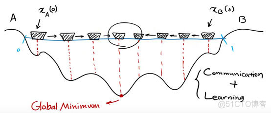
一个较大的惯性权重有利于全局搜索，而一个较小的惯性权重则更利于局部搜索。接下来先对惯性权重进行修改，总共有两种类型：线性递减惯性权重(LDIW)和非线性递减惯性权重。

线性递减惯性权重

将惯性权重 w w w从一个常数变为以下公式：

w d = w s t a r t − ( w s t a r t − w e n d ) × d K w^d=w_{start}-(w_{start}-w_{end})×\frac{d}{K} wd=​−(​−wend​)×Kd​

其中 d d d是循环次数， K K K是总共的循环次数。

非线性递减惯性权重

常见的有以下两种方法：

w d = w s t a r t − ( w s t a r t − w e n d ) × ( d K ) 2 w^d=w_{start}-(w_{start}-w_{end})×{\left(\frac{d}{K}\right)}^2 wd=​−(​−wend​)×(Kd​)2 w d = w s t a r t − ( w s t a r t − w e n d ) × [ 2 d K − ( d K ) 2 ] w^d=w_{start}-(w_{start}-w_{end})×\left[\frac{2d}{K}-{\left(\frac{d}{K}\right)}^2\right] wd=​−(​−wend​)×[K2d​−(Kd​)2] 绘制出三种惯性权重修改式的曲线 代码

import numpy as np
import matplotlib.pyplot as plt# 初始化PSO参数
x = np.linspace(0,49,50)
w_start = 0.9
w_end = 0.1
K = 50 # 循环次数w0 = w_start - (w_start-w_end)*(x/K) # 线性递减惯性权重
w1 = w_start - (w_start-w_end)*(x/K)**2 # 非线性递减惯性权重1
w2 = w_start - (w_start-w_end)*(2*(x/K)-(x/K)**2) # 非线性递减惯性权重2fig,ax = plt.subplots()
plt.rcParams['font.sans-serif']=['SimHei'] #用来正常显示中文标签
ax.plot(x,w0,label = '线性递减惯性权重')
ax.plot(x,w1,label = '非线性递减惯性权重1')
ax.plot(x,w2,label = '非线性递减惯性权重2')
ax.legend()

绘制结果

使用线性递减惯性权重求解二元函数的最值问题 题目

求函数 y = x 1 2 + x 2 2 − x 1 x 2 − 10 x 1 − 4 x 2 + 60 y =x_1^2+x_2^2--10x_1-4x_2+60 y=x12​+x22​−x1​x2​−10x1​−4x2​+60在 x 1 , x 2 ∈ [ − 15 , 15 ] x_1,x_2∈[-15,15] x1​,x2​∈[−15,15]内的最小值。流程图

代码实现

# 第一步，绘制函数图像
# 第一步，绘制函数图像
import numpy as np
import matplotlib.pyplot as plt
import mpl_toolkits.mplot3ddef func(x,y):return x**2+y**2-x*y-10*x-4*y+60x0 = np.linspace(-15,15,100)
y0 = np.linspace(-15,15,100)
x0,y0 = np.meshgrid(x0,y0)
z0 = func(x0,y0)
fig = plt.figure(constrained_layout=True)
ax = fig.add_subplot(projection='3d')
ax.plot_surface(x0,y0,z0,cmap=plt.cm.viridis,alpha=0.7)
#ax.plot_wireframe(x0,y0,z0) # 另一种绘图方式
ax.set_title('$y = x_1^2+x_2^2-x_1x_2-10x_1-4x_2+60$')# 第二步，设置粒子群算法的参数
n = 30 # 粒子数量
narvs = 2 # 变量个数
c1 = 2 # 个体学习因子
c2 = 2 # 社会学习因子
w_start = 0.9 # 惯性权重
w_end = 0.1
K = 40 # 迭代次数
vxmax = np.array([(15-(-15))*0.2,(15-(-15))*0.2]) # 粒子在x方向的最大速度
x_lb = np.array([-15,-15]) # x和y的下界
x_ub = np.array([15,15]) # x和y的上界# 第三步，初始化粒子   
x = x_lb + (x_ub-x_lb)*np.random.rand(n,narvs)
v = -vxmax + 2*vxmax*np.random.rand(n,narvs)# 第四步，计算适应度
fit = func(x[:,0],x[:,1]) # 计算每个粒子的适应度
pbest = x # 初始化这n个例子迄今为止找到的最佳位置
ind = np.argmax(fit) # 找到适应度最大的那个粒子的下标
gbest = x[ind,:]
gbest_total = np.zeros(K)# 第五步，更新粒子速度和位置
for j in range(K): # 外层循环，共K次w = w_start - (w_start-w_end)*(j/K) # 修改后的惯性权重表达式for p in range(n):v[p,:] = w*v[p,:] + c1*np.random.rand(narvs)*(pbest[p,:]-x[p,:]) + c2*np.random.rand(narvs)*(gbest-x[p,:])loc_v = np.where(v<-vxmax)v[loc_v] = -vxmax[loc_v[1]] # 速度小于-vmax的元素赋值为-vmaxloc_v = np.where(v>vxmax)v[loc_v] = vxmax[loc_v[1]] # 速度大于vmax的元素赋值为vmaxx = x + v # 更新第i个粒子的位置loc_x = np.where(x<x_lb)x[loc_x] = x_lb[loc_x[1]]loc_x = np.where(x>x_ub)x[loc_x] = x_ub[loc_x[1]]# 第六步，重新计算适应度并找到最优粒子fit = func(x[:,0],x[:,1]) # 重新计算n个粒子的适应度for k in range(n): # 更新第k个粒子迄今为止找到的最佳位置if fit[k]<func(pbest[k,0],pbest[k,1]):pbest[k,:] = x[k,:]if np.min(fit)<func(gbest[0],gbest[1]): # 更新所有粒子迄今找到的最佳位置gbest = x[np.argmin(fit),:]gbest_total[j] = func(gbest[0],gbest[1])ax.scatter(x[:,0],x[:,1],fit,c='r',marker='x')
fig,ax = plt.subplots()
ax.plot(np.arange(K),gbest_total)
plt.rcParams['font.sans-serif']=['SimHei'] #用来正常显示中文标签
plt.rcParams['axes.unicode_minus'] = False #用来显示负号
ax.set_title('算法找到的最小值随优化次数的变化曲线')
ax.set_xlabel('循环次数')
ax.autoscale(axis='x',tight=True)
print('找到的最优解为：',func(gbest[0],gbest[1]))

绘制结果 使用非线性递减惯性权重1求解二元函数的最值问题 权重公式：

w d = w s t a r t − ( w s t a r t − w e n d ) × ( d K ) 2 w^d=w_{start}-(w_{start}-w_{end})×{\left(\frac{d}{K}\right)}^2 wd=​−(​−wend​)×(Kd​)代码

# 第一步，绘制函数图像
import numpy as np
import matplotlib.pyplot as plt
import mpl_toolkits.mplot3ddef func(x,y):return x**2+y**2-x*y-10*x-4*y+60x0 = np.linspace(-15,15,100)
y0 = np.linspace(-15,15,100)
x0,y0 = np.meshgrid(x0,y0)
z0 = func(x0,y0)
fig = plt.figure(constrained_layout=True)
ax = fig.add_subplot(projection='3d')
ax.plot_surface(x0,y0,z0,cmap=plt.cm.viridis,alpha=0.7)
#ax.plot_wireframe(x0,y0,z0) # 另一种绘图方式
ax.set_title('$y = x_1^2+x_2^2-x_1x_2-10x_1-4x_2+60$')# 第二步，设置粒子群算法的参数
n = 30 # 粒子数量
narvs = 2 # 变量个数
c1 = 2 # 个体学习因子
c2 = 2 # 社会学习因子
w_start = 0.9 # 惯性权重
w_end = 0.1
K = 40 # 迭代次数
vxmax = np.array([(15-(-15))*0.2,(15-(-15))*0.2]) # 粒子在x方向的最大速度
x_lb = np.array([-15,-15]) # x和y的下界
x_ub = np.array([15,15]) # x和y的上界# 第三步，初始化粒子   
x = x_lb + (x_ub-x_lb)*np.random.rand(n,narvs)
v = -vxmax + 2*vxmax*np.random.rand(n,narvs)# 第四步，计算适应度
fit = func(x[:,0],x[:,1]) # 计算每个粒子的适应度
pbest = x # 初始化这n个例子迄今为止找到的最佳位置
ind = np.argmax(fit) # 找到适应度最大的那个粒子的下标
gbest = x[ind,:]
gbest_total = np.zeros(K)# 第五步，更新粒子速度和位置
for j in range(K): # 外层循环，共K次w = w_start - (w_start-w_end)*(j/K)**2 # 修改后的惯性权重表达式for p in range(n):v[p,:] = w*v[p,:] + c1*np.random.rand(narvs)*(pbest[p,:]-x[p,:]) + c2*np.random.rand(narvs)*(gbest-x[p,:])loc_v = np.where(v<-vxmax)v[loc_v] = -vxmax[loc_v[1]] # 速度小于-vmax的元素赋值为-vmaxloc_v = np.where(v>vxmax)v[loc_v] = vxmax[loc_v[1]] # 速度大于vmax的元素赋值为vmaxx = x + v # 更新第i个粒子的位置loc_x = np.where(x<x_lb)x[loc_x] = x_lb[loc_x[1]]loc_x = np.where(x>x_ub)x[loc_x] = x_ub[loc_x[1]]# 第六步，重新计算适应度并找到最优粒子fit = func(x[:,0],x[:,1]) # 重新计算n个粒子的适应度for k in range(n): # 更新第k个粒子迄今为止找到的最佳位置if fit[k]<func(pbest[k,0],pbest[k,1]):pbest[k,:] = x[k,:]if np.min(fit)<func(gbest[0],gbest[1]): # 更新所有粒子迄今找到的最佳位置gbest = x[np.argmin(fit),:]gbest_total[j] = func(gbest[0],gbest[1])ax.scatter(x[:,0],x[:,1],fit,c='r',marker='x')
fig.savefig('./program8.png',dpi=500)
fig,ax = plt.subplots()
ax.plot(np.arange(K),gbest_total)
plt.rcParams['font.sans-serif']=['SimHei'] #用来正常显示中文标签
plt.rcParams['axes.unicode_minus'] = False #用来显示负号
ax.set_title('算法找到的最小值随优化次数的变化曲线')
ax.set_xlabel('循环次数')
ax.autoscale(axis='x',tight=True)
print('找到的最优解为：',func(gbest[0],gbest[1]))
fig.savefig('./program9.png',dpi=500)

绘制结果 使用非线性递减惯性权重2求解二元函数的最值问题 权重公式：

w d = w s t a r t − ( w s t a r t − w e n d ) × [ 2 d K − ( d K ) 2 ] w^d=w_{start}-(w_{start}-w_{end})×\left[\frac{2d}{K}-{\left(\frac{d}{K}\right)}^2\right] wd=​−(​−wend​)×[K2d​−(Kd​)2]代码

# 第一步，绘制函数图像
import numpy as np
import matplotlib.pyplot as plt
import mpl_toolkits.mplot3ddef func(x,y):return x**2+y**2-x*y-10*x-4*y+60x0 = np.linspace(-15,15,100)
y0 = np.linspace(-15,15,100)
x0,y0 = np.meshgrid(x0,y0)
z0 = func(x0,y0)
fig = plt.figure(constrained_layout=True)
ax = fig.add_subplot(projection='3d')
ax.plot_surface(x0,y0,z0,cmap=plt.cm.viridis,alpha=0.7)
#ax.plot_wireframe(x0,y0,z0) # 另一种绘图方式
ax.set_title('$y = x_1^2+x_2^2-x_1x_2-10x_1-4x_2+60$')# 第二步，设置粒子群算法的参数
n = 30 # 粒子数量
narvs = 2 # 变量个数
c1 = 2 # 个体学习因子
c2 = 2 # 社会学习因子
w_start = 0.9 # 惯性权重
w_end = 0.1
K = 40 # 迭代次数
vxmax = np.array([(15-(-15))*0.2,(15-(-15))*0.2]) # 粒子在x方向的最大速度
x_lb = np.array([-15,-15]) # x和y的下界
x_ub = np.array([15,15]) # x和y的上界# 第三步，初始化粒子   
x = x_lb + (x_ub-x_lb)*np.random.rand(n,narvs)
v = -vxmax + 2*vxmax*np.random.rand(n,narvs)# 第四步，计算适应度
fit = func(x[:,0],x[:,1]) # 计算每个粒子的适应度
pbest = x # 初始化这n个例子迄今为止找到的最佳位置
ind = np.argmax(fit) # 找到适应度最大的那个粒子的下标
gbest = x[ind,:]
gbest_total = np.zeros(K)# 第五步，更新粒子速度和位置
for j in range(K): # 外层循环，共K次w = w_start - (w_start-w_end)*(2*(j/K)-(j/K)**2) # 修改后的惯性权重表达式for p in range(n):v[p,:] = w*v[p,:] + c1*np.random.rand(narvs)*(pbest[p,:]-x[p,:]) + c2*np.random.rand(narvs)*(gbest-x[p,:])loc_v = np.where(v<-vxmax)v[loc_v] = -vxmax[loc_v[1]] # 速度小于-vmax的元素赋值为-vmaxloc_v = np.where(v>vxmax)v[loc_v] = vxmax[loc_v[1]] # 速度大于vmax的元素赋值为vmaxx = x + v # 更新第i个粒子的位置loc_x = np.where(x<x_lb)x[loc_x] = x_lb[loc_x[1]]loc_x = np.where(x>x_ub)x[loc_x] = x_ub[loc_x[1]]# 第六步，重新计算适应度并找到最优粒子fit = func(x[:,0],x[:,1]) # 重新计算n个粒子的适应度for k in range(n): # 更新第k个粒子迄今为止找到的最佳位置if fit[k]<func(pbest[k,0],pbest[k,1]):pbest[k,:] = x[k,:]if np.min(fit)<func(gbest[0],gbest[1]): # 更新所有粒子迄今找到的最佳位置gbest = x[np.argmin(fit),:]gbest_total[j] = func(gbest[0],gbest[1])ax.scatter(x[:,0],x[:,1],fit,c='r',marker='x')
fig,ax = plt.subplots()
ax.plot(np.arange(K),gbest_total)
plt.rcParams['font.sans-serif']=['SimHei'] #用来正常显示中文标签
plt.rcParams['axes.unicode_minus'] = False #用来显示负号
ax.set_title('算法找到的最小值随优化次数的变化曲线')
ax.set_xlabel('循环次数')
ax.autoscale(axis='x',tight=True)
print('找到的最优解为：',func(gbest[0],gbest[1]))

绘制结果