[Hands On ML] 2. 一个完整的机器学习项目(加州房价预测)
文章目录 10. 自定义转换器11. 特征缩放12. 转换流水线. 训练模型14. 交叉验证15. 微调模型 16. 分析最佳模型的误差17. 用测试集评估模型18. 启动、监控、维护系统19. 练习
本文为《机器学习实战:基于-Learn和》的读书笔记。
中文翻译参考
1. 项目介绍
利用加州普查数据,建立一个加州房价模型。
数据包含每个街区组的人口、收入中位数、房价中位数等指标。
利用这个数据进行学习,然后根据其它指标,预测任何街区的的房价中位数。
2. 性能指标
均方根误差(RMSE):
RMSE ( X , h ) = 1 m ∑ i = 1 m ( h ( x ( i ) ) − y ( i ) ) 2 \{RMSE}(\{X}, h)=\sqrt{\frac{1}{m} \sum\{i=1}^{m}\left(h\left(\{x}^{(i)}\right)-y^{(i)}\right)^{2}} RMSE(X,h)=m1i=1∑m(h(x(i))−y(i))2
平均绝对误差(MAE)
MAE ( X , h ) = 1 m ∑ i = 1 m ∣ h ( x ( i ) ) − y ( i ) ∣ \{MAE}(\{X}, h)=\frac{1}{m} \sum\{i=1}^{m}\left|h\left(\{x}^{(i)}\right)-y^{(i)}\right| MAE(X,h)=m1i=1∑m∣∣∣h(x(i))−y(i)∣∣∣
范数的指数越高,就越关注大的值而忽略小的值。这就是为什么 RMSE 比 MAE 对异常值更敏感。但是当异常值是指数分布的(类似正态曲线),RMSE 就会表现很好。
3. 确定任务类型
是分类?(房子便宜、中等、昂贵)
是回归?(预测房子价格),本任务是回归。
4. 查看数据
import pandas as pd
data = pd.read_csv("housing.csv")
data.info()
<class 'pandas.core.frame.DataFrame'>
RangeIndex: 20640 entries, 0 to 20639
Data columns (total 10 columns):
longitude             20640 non-null float64
latitude              20640 non-null float64
housing_median_age    20640 non-null float64
total_rooms           20640 non-null float64
total_bedrooms        20433 non-null float64
population            20640 non-null float64
households            20640 non-null float64
median_income         20640 non-null float64
median_house_value    20640 non-null float64
ocean_proximity       20640 non-null object
dtypes: float64(9), object(1)
memory usage: 1.6+ MB
20433 non-null 有缺失数据
data['ocean_proximity'].value_counts()
查看 ocean_proximity 特征 有多少种值
<1H OCEAN     9136
INLAND        6551
NEAR OCEAN    2658
NEAR BAY      2290
ISLAND           5
Name: ocean_proximity, dtype: int64
data.describe()
数字特征统计
data.head()
数据前5行
%matplotlib inline
import matplotlib.pyplot as plt
data.hist(bins=50,figsize=(20,15))
直方图
数据有不同的量纲,一些数据左右分布不均匀。一般将其变为正态分布,一些模型会工作的比较好。
5. 创建测试集
from sklearn.model_selection import train_test_split
train_set, test_set = train_test_split(data, test_size=0.2, random_state=1)
train_set.info()
<class 'pandas.core.frame.DataFrame'>
Int64Index: 16512 entries, 15961 to 235
Data columns (total 10 columns):
longitude             16512 non-null float64
latitude              16512 non-null float64
housing_median_age    16512 non-null float64
total_rooms           16512 non-null float64
total_bedrooms        16349 non-null float64
population            16512 non-null float64
households            16512 non-null float64
median_income         16512 non-null float64
median_house_value    16512 non-null float64
ocean_proximity       16512 non-null object
dtypes: float64(9), object(1)
memory usage: 1.4+ MB
这种随机的切分方法,在数据量小的时候可能会出现,分出来的数据某些特征比例不再是原有的比例,后序预测可能造成误差
import numpy as np
data['income_cat'] = np.ceil(data['median_income']/1.5)
data['income_cat']
data['income_cat'].where(data['income_cat'] < 5, 5.0, inplace=True)
# pd.where() Where cond is True, keep the original value.
# Where False, replace with corresponding value from other
大于等于 5 的, 替换成 5, 把收入分成几类
data['income_cat'].hist()
data['income_cat'].value_counts()/len(data)
3.0    0.350581
2.0    0.318847
4.0    0.176308
5.0    0.114438
1.0    0.039826
Name: income_cat, dtype: float64
from sklearn.model_selection import StratifiedShuffleSplit
# help(StratifiedShuffleSplit)
splt = StratifiedShuffleSplit(n_splits=1, test_size=0.2, random_state=1)
for train_idx, test_idx in splt.split(data, data['income_cat']): # 按照后者分层抽样strat_train_set = data.loc[train_idx]strat_test_set = data.loc[test_idx]# 查看分布
strat_train_set['income_cat'].value_counts()/len(strat_train_set)
strat_test_set['income_cat'].value_counts()/len(strat_test_set)
查看抽样结果,跟上面原始数据的分布很接近
3.0    0.350533
2.0    0.318798
4.0    0.176357
5.0    0.114583
1.0    0.039729
Name: income_cat, dtype: float64
分层采样的收入分类比例与总数据集几乎相同,而随机采样数据集偏差严重
删除新增列,回到初始数据状态
for set in (strat_train_set, strat_test_set):set.drop('income_cat',axis=1, inplace=True)
strat_train_set
6. 数据可视化
housing = strat_train_set.copy() # 复制避免损坏
housing.plot(kind='scatter',x='longitude',y='latitude')
# 调整alpha,可以看出密度差异
housing.plot(kind='scatter',x='longitude',y='latitude',alpha=0.1)
housing.plot(kind='scatter',x='longitude',y='latitude',alpha=0.4,s=housing['population']/100, label='population',c='median_house_value',cmap=plt.get_cmap('jet'))
每个圈的半径表示街区的人口(选项s),颜色代表价格(选项c)
可以看出,距离海岸近的房价较高,但是北边海岸边的价格又不是很高
7. 查找数据关联
相关系数
corr_mat = housing.corr()
corr_mat
corr_mat['median_house_value'].sort_values(ascending=False)
median_house_value    1.000000
median_income         0.684828
total_rooms           0.133566
housing_median_age    0.107684
households            0.065778
total_bedrooms        0.049941
population           -0.025008
longitude            -0.043824  # 经度,东西
latitude             -0.146748	# 纬度,南北
Name: median_house_value, dtype: float64
可以看到纬度越大(北边),房价(越低),呈负相关
attributes = ["median_house_value", "median_income", "total_rooms", "housing_median_age"]
pd.plotting.scatter_matrix(housing[attributes],figsize=(12,8))
挑几个可能跟房价先关的特征出来,画出相关性图
可以看出收入的中位数特征,最有可能用来预测房价,将该子图放大
housing.plot(kind='scatter',x='median_income',y='median_house_value',alpha=0.1)
8. 特征组合
数据在交给算法之前,最后一件事是尝试多种属性组合
例如,如果你不知道某个街区有多少户,该街区的总房间数就没什么用。你真正需要的是每户有几个房间。
相似的,总卧室数也不重要:你可能需要将其与房间数进行比较。每户的人口数也是一个有趣的属性组合。
# 每家的房间数
housing["rooms_per_household"] = housing["total_rooms"]/housing["households"]
# 每家的卧室数量比
housing["bedrooms_per_room"] = housing["total_bedrooms"]/housing["total_rooms"]
# 每家的人口
housing["population_per_household"]=housing["population"]/housing["households"]corr_mat = housing.corr()
corr_mat['median_house_value'].sort_values(ascending=False)
median_house_value          1.000000
median_income               0.684828
rooms_per_household         0.171947  # 新特征1
total_rooms                 0.133566  # 1a  3b
housing_median_age          0.107684
households                  0.065778  # 1b  2b
total_bedrooms              0.049941  # 3a
population                 -0.025008  # 2a
population_per_household   -0.026596  # 新特征2
longitude                  -0.043824
latitude                   -0.146748
bedrooms_per_room          -0.256396  # 新特征3
Name: median_house_value, dtype: float64
可以看出新的特征比原特征,与房价之间有更高的相关性
9. 为算法准备数据
尽量写一些函数来处理,以便复用,代码也更清晰
分离 特征 与 标签
housing = strat_train_set.drop('median_house_value',axis=1)
housing_label = strat_train_set['median_house_value'].copy()
9.1 数据清洗
有缺失,可以:
housing.dropna(subset=["total_bedrooms"])    # 选项1
housing.drop("total_bedrooms", axis=1)       # 选项2
median = housing["total_bedrooms"].median()	 记得保存,后序填补test集
housing["total_bedrooms"].fillna(median)    # 选项3
from sklearn.impute import SimpleImputer
impter = SimpleImputer(strategy='median')
# 数值属性才能计算中位数
housing_num = housing.drop('ocean_proximity',axis=1)
impter.fit(housing_num)
impter.statistics_
array([-118.49 , 34.26 , 29. , 2122.5 , 434. ,1163. , 409. , 3.52945])
housing_num.median().values
跟上面一样
array([-118.49   ,   34.26   ,   29.     , 2122.5    ,  434.     ,1163.     ,  409.     ,    3.52945])
应用转换,填补确实数据为中位数
X = impter.transform(housing_num)
type(X) # numpy.ndarray
转换完为 numpy 数组,再转回
housing_tr = pd.DataFrame(X, columns=housing_num.columns)
type(housing_tr)  # pandas.core.frame.DataFrame
9.2 处理文本特征
from sklearn.preprocessing import LabelEncoder
encoder = LabelEncoder() # 只能对第一文本列,多文本列使用pd.factorize()
housing_cat = housing['ocean_proximity']
housing_cat_encoded = encoder.fit_transform(housing_cat)
housing_cat_encoded
print(encoder.classes_)
['<1H OCEAN' 'INLAND' 'ISLAND' 'NEAR BAY' 'NEAR OCEAN']
这样做,标签对应于 0,1,2,算法在计算距离相似度的时候,会产生偏差:(0,4显然比0,1更相似)
采用 独热编码(One-Hot ),只有一个属性会等于 1(热),其余会是 0(冷),计算距离相似度的时候更合理
from sklearn.preprocessing import OneHotEncoder
encoder = OneHotEncoder()
housing_cat_1hot = encoder.fit_transform(housing_cat_encoded.reshape(-1,1))
注意:需要单列数据需要 reshape(-1,1),转成矩阵
housing_cat_1hot
<16512x5 sparse matrix of type 'numpy.float64'>'with 16512 stored elements in Compressed Sparse Row format>
输出结果是一个 SciPy 稀疏矩阵,而不是 NumPy 数组。
housing_cat_1hot.toarray()array([[0., 0., 0., 1., 0.],[0., 1., 0., 0., 0.],[1., 0., 0., 0., 0.],...,[1., 0., 0., 0., 0.],[0., 1., 0., 0., 0.],[0., 1., 0., 0., 0.]])
from sklearn.preprocessing import LabelBinarizer
encoder = LabelBinarizer()向构造器LabelBinarizer传递 sparse_output=True,就可以得到一个稀疏矩阵
housing_cat_1hot = encoder.fit_transform(housing_cat)
housing_cat_1hotarray([[0, 0, 0, 1, 0],[0, 1, 0, 0, 0],[1, 0, 0, 0, 0],...,[1, 0, 0, 0, 0],[0, 1, 0, 0, 0],[0, 1, 0, 0, 0]])
10. 自定义转换器
创建一个类并执行三个方法:fit()(返回self),(),和()
from sklearn.base import BaseEstimator, TransformerMixin
rooms_ix, bedrooms_ix, population_ix, household_ix = 3, 4, 5, 6class CombinedAttributesAdder(BaseEstimator, TransformerMixin):def __init__(self, add_bedrooms_per_room = True): # no *args or **kargsself.add_bedrooms_per_room = add_bedrooms_per_roomdef fit(self, X, y=None):return self  # nothing else to dodef transform(self, X, y=None):rooms_per_household = X[:, rooms_ix] / X[:, household_ix]population_per_household = X[:, population_ix] / X[:, household_ix]if self.add_bedrooms_per_room:bedrooms_per_room = X[:, bedrooms_ix] / X[:, rooms_ix]return np.c_[X, rooms_per_household, population_per_household,bedrooms_per_room]else:return np.c_[X, rooms_per_household, population_per_household]attr_adder = CombinedAttributesAdder(add_bedrooms_per_room=False)
housing_extra_attribs = attr_adder.transform(housing.values)
housing_extra_attribsarray([[-122.13, 37.67, 40.0, ..., 'NEAR BAY', 5.514195583596215,2.8832807570977916],[-120.98, 37.65, 40.0, ..., 'INLAND', 6.698412698412699,2.507936507936508],[-118.37, 33.87, 23.0, ..., '<1H OCEAN', 5.137640449438202,2.502808988764045],...,[-117.69, 33.58, 5.0, ..., '<1H OCEAN', 6.80040733197556,2.9297352342158858],[-117.3, 34.1, 49.0, ..., 'INLAND', 4.615384615384615,5.846153846153846],[-121.77, 37.99, 4.0, ..., 'INLAND', 7.853351955307263,3.392458100558659]], dtype=object)
11. 特征缩放
不同的特征量纲不一样,在基于距离的机器学习算法中,特征的权重不一样,会造成误差
线性函数归一化(归一化())很简单:通过减去最小值,然后再除以最大值与最小值的差值,来进行归一化。
标准化:先减去平均值(所以标准化值的平均值总是 0),然后除以方差,使得到的分布具有单位方差。
警告:与所有的转换一样,缩放器只能向训练集拟合,而不是向完整的数据集(包括测试集)。只有这样,你才能用缩放器转换训练集和测试集(和新数据)。
12. 转换流水线
存在许多数据转换步骤,需要按一定的顺序执行。-Learn 提供了类,来进行这一系列的转换。
from sklearn.pipeline import Pipeline
from sklearn.preprocessing import StandardScalernum_pipeline = Pipeline([('imputer',SimpleImputer(strategy='median')),('attibs_adder',CombinedAttributesAdder()),('std_scaler',StandardScaler()),
])
housing_num_tr = num_pipeline.fit_transform(housing_num)
housing_num_trarray([[-1.27826235,  0.95445204,  0.89646428, ...,  0.04435599,-0.01693693, -0.49175254],[-0.70432019,  0.94509343,  0.89646428, ...,  0.56563549,-0.05135459, -0.99646009],[ 0.59827896, -0.82368426, -0.45394013, ..., -0.12139949,-0.05182477, -0.5064297 ],...,[ 0.93765346, -0.95938413, -1.88378009, ...,  0.61053242,-0.01267723, -0.96392659],[ 1.13229471, -0.71606022,  1.61138426, ..., -0.35129083,0.25474742, -0.46992773],[-1.0985935 ,  1.10418984, -1.96321564, ...,  1.0740272 ,0.02975272, -1.15998515]])
构造器需要一个定义步骤顺序的名字/估计器对的列表
除了最后一个估计器,其余都要是转换器(它们都要有()方法)。名字随意起
调用流水线的fit()方法,会对所有转换器顺序调用()方法,将每次调用的输出作为参数传递给下一个调用
一直到最后一个估计器,它只执行fit()方法
流水线暴露相同的方法作为最终的估计器。在这个例子中,最后的估计器是一个,它是一个转换器,因此这个流水线有一个()方法,可以顺序对数据做所有转换(它还有一个方法可以使用,就不必先调用fit()再进行())
如果不需要手动将中的数值列转成Numpy数组的格式,而可以直接将输入中进行处理就好了。
-Learn 没有工具来处理 ,因此我们需要写一个简单的自定义转换器来做这项工作:
from sklearn.base import BaseEstimator, TransformerMixinclass DataFrameSelector(BaseEstimator, TransformerMixin):def __init__(self,attribute_names):self.attribute_names = attribute_namesdef fit(self,X,y=None):return selfdef transform(self,X):return X[self.attribute_names].values
# 报错参考 https://blog.csdn.net/jasonzhoujx/article/details/82025571
class MyLabelBinarizer(TransformerMixin):def __init__(self, *args, **kwargs):self.encoder = LabelBinarizer(*args, **kwargs)def fit(self, x, y=0):self.encoder.fit(x)return selfdef transform(self, x, y=0):return self.encoder.transform(x)from sklearn.pipeline import FeatureUnion
num_attribs = list(housing_num)
cat_attribs = ["ocean_proximity"]num_pipeline = Pipeline([('selector',DataFrameSelector(num_attribs)),('Simpleimputer', SimpleImputer(strategy="median")),('attribs_adder', CombinedAttributesAdder()),('std_scaler', StandardScaler()),
])cat_pipeline = Pipeline([('selector',DataFrameSelector(cat_attribs)),('label_binarizer',MyLabelBinarizer())
])full_pipeline = FeatureUnion(transformer_list=[('num_pipeline',num_pipeline),('cat_pipeline',cat_pipeline),
])
# help(FeatureUnion)housing_prepared = full_pipeline.fit_transform(housing)
housing_preparedarray([[-1.27826235,  0.95445204,  0.89646428, ...,  0.        ,1.        ,  0.        ],[-0.70432019,  0.94509343,  0.89646428, ...,  0.        ,0.        ,  0.        ],[ 0.59827896, -0.82368426, -0.45394013, ...,  0.        ,0.        ,  0.        ],...,[ 0.93765346, -0.95938413, -1.88378009, ...,  0.        ,0.        ,  0.        ],[ 1.13229471, -0.71606022,  1.61138426, ...,  0.        ,0.        ,  0.        ],[-1.0985935 ,  1.10418984, -1.96321564, ...,  0.        ,0.        ,  0.        ]])
13. 训练模型
初步选择 线性回归模型
from sklearn.linear_model import LinearRegression
lin_reg = LinearRegression()
lin_reg.fit(housing_prepared, housing_label)somedata = housing.iloc[:5]
somelabel = housing_label.iloc[:5]
somedata_prepared = full_pipeline.transform(somedata)
print('predict:\t', lin_reg.predict(somedata_prepared))
print('Labels:\t',list(somelabel))predict:	 [234956.84260842 303073.513104   327746.46204573 355932.30741583210220.50294171]
Labels:	 [184000.0, 172200.0, 359900.0, 258200.0, 239100.0]
from sklearn.metrics import mean_squared_error
housing_predict = lin_reg.predict(housing_prepared)
lin_mse = mean_squared_error(housing_predict, housing_label)
lin_rmse = np.sqrt(lin_mse)
lin_rmse68860.85279166883
误差很大,效果不是很理想
模型欠拟合:
修复欠拟合的主要方法:
先让我们尝试一个更为复杂的模型,看看效果。
来训练一个r。这是一个强大的模型,可以发现数据中复杂的非线性关系
from sklearn.tree import DecisionTreeRegressortree_reg = DecisionTreeRegressor()
tree_reg.fit(housing_prepared, housing_label)housing_predictions = tree_reg.predict(housing_prepared)
tree_mse = mean_squared_error(housing_label, housing_predictions)
tree_rmse = np.sqrt(tree_mse)
tree_rmse误差 0.0,太强了? 错了,上面使用了全部的训练集训练,然后在训练集上预测,产生了过拟合
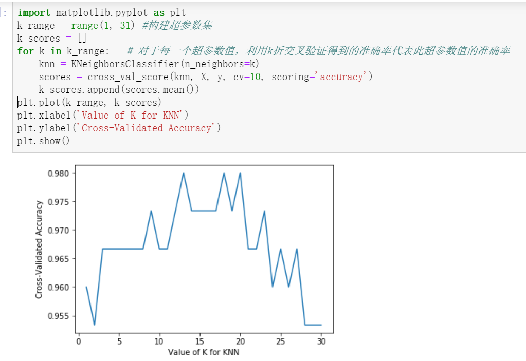
14. 交叉验证
K 折交叉验证(K-fold cross-):
from sklearn.model_selection import cross_val_score
scores = cross_val_score(tree_reg,housing_prepared,housing_label,scoring='neg_mean_squared_error', cv=10)
tree_rmse_scores = np.sqrt(-scores) # sklearn用的是负数
print(tree_rmse_scores)
print(tree_rmse_scores.mean())
print(tree_rmse_scores.std())[71214.4929498  71929.79930468 70914.76077221 69550.7256691271042.25558966 67279.14165025 73061.35854347 71568.8525624271380.99149371 69504.81637098]
70744.71949063087
1522.0580698181013
再用 线性回归 模型,试下交叉验证的结果
lin_scores = cross_val_score(lin_reg, housing_prepared, housing_label,scoring='neg_mean_squared_error', cv=10)
lin_rmse_scores = np.sqrt(-lin_scores)
print(lin_rmse_scores)
print(lin_rmse_scores.mean())
print(lin_rmse_scores.std())[70987.24786319 66375.29508519 73837.53789445 69493.5958464269821.05544742 69047.06162451 65908.72602507 66979.3303266973036.00622233 67077.50225384]
69256.33585891136
2610.121268165482
再试下 随机森林 模型
from sklearn.ensemble import RandomForestRegressor
forest_reg = RandomForestRegressor()
forest_scores = cross_val_score(forest_reg,housing_prepared,housing_label,scoring='neg_mean_squared_error',cv=10)
forest_rmse_scores = np.sqrt(-forest_scores)
print(forest_rmse_scores)
print(forest_rmse_scores.mean())
print(forest_rmse_scores.std())[51968.86058788 47122.75805482 48941.3492676  50877.9942948951200.95320051 49198.87467112 49401.27484477 48418.5361811553788.16232918 49438.88539583]
50035.76488277516
1834.1856707471993
随机森林模型,比上面2个模型得到的结果的误差要小。看起来是个不错的选择。
在深入随机森林之前,应该尝试下机器学习算法的其它类型模型(不同核的支持向量机,神经网络,等等),不要在调节超参数上花费太多时间。目标是列出一个可能模型的列表(两到五个)。
提示:要保存每个试验过的模型,以便后续可以再用。
要确保有超参数和训练参数,以及交叉验证评分,和实际的预测值。
这可以让你比较不同类型模型的评分,还可以比较误差种类。
你可以用 的模块 ,非常方便地保存 -Learn 模型,或使用 ..,后者序列化大 NumPy 数组更有效率
from sklearn.externals import joblib
joblib.dump(forest_reg, "my_forest.pkl")
my_forest_model = joblib.load("my_forest.pkl")
15. 微调模型
假设有几个有希望的模型。现在需要对它们进行微调
15.1 网格搜索
你应该使用 -Learn 的 来做这项搜索工作
from sklearn.model_selection import GridSearchCVparam_grid = [{'n_estimators' : [3,10,30],'max_features':[2,4,6,8]},{'bootstrap':[False], 'n_estimators' : [3,10],'max_features':[2,3,4]},
]
forest_reg = RandomForestRegressor()
grid_search = GridSearchCV(forest_reg, param_grid, cv=5,scoring='neg_mean_squared_error')
grid_search.fit(housing_prepared, housing_label)#----------------------------------
GridSearchCV(cv=5, error_score=nan,estimator=RandomForestRegressor(bootstrap=True, ccp_alpha=0.0,criterion='mse', max_depth=None,max_features='auto',max_leaf_nodes=None,max_samples=None,min_impurity_decrease=0.0,min_impurity_split=None,min_samples_leaf=1,min_samples_split=2,min_weight_fraction_leaf=0.0,n_estimators=100, n_jobs=None,oob_score=False, random_state=None,verbose=0, warm_start=False),iid='deprecated', n_jobs=None,param_grid=[{'max_features': [2, 4, 6, 8],'n_estimators': [3, 10, 30]},{'bootstrap': [False], 'max_features': [2, 3, 4],'n_estimators': [3, 10]}],pre_dispatch='2*n_jobs', refit=True, return_train_score=False,scoring='neg_mean_squared_error', verbose=0)
完成后,你就能获得参数的最佳组合
grid_search.best_params_{'max_features': 8, 'n_estimators': 30}
注意到参数在边界上,可能还要继续扩大范围搜索
最佳的模型
grid_search.best_estimator_
#---------output-------------
RandomForestRegressor(bootstrap=True, ccp_alpha=0.0, criterion='mse',max_depth=None, max_features=8, max_leaf_nodes=None,max_samples=None, min_impurity_decrease=0.0,min_impurity_split=None, min_samples_leaf=1,min_samples_split=2, min_weight_fraction_leaf=0.0,n_estimators=30, n_jobs=None, oob_score=False,random_state=None, verbose=0, warm_start=False)
cv_result = grid_search.cv_results_
for mean_score, params in zip(cv_result['mean_test_score'], cv_result['params']):print(np.sqrt(-mean_score), params)
. 包含的内容:
cv_result = grid_search.cv_results_
for mean_score, params in zip(cv_result['mean_test_score'], cv_result['params']):print(np.sqrt(-mean_score), params)18 种模型参数下的模型表现
65764.17270897377 {'max_features': 2, 'n_estimators': 3}
55028.13746266011 {'max_features': 2, 'n_estimators': 10}
53074.92097234033 {'max_features': 2, 'n_estimators': 30}
59883.77893095 {'max_features': 4, 'n_estimators': 3}
53191.69949879354 {'max_features': 4, 'n_estimators': 10}
50181.08262957352 {'max_features': 4, 'n_estimators': 30}
58994.29777449576 {'max_features': 6, 'n_estimators': 3}
52167.31741521162 {'max_features': 6, 'n_estimators': 10}
50241.45200619339 {'max_features': 6, 'n_estimators': 30}
58312.46978517355 {'max_features': 8, 'n_estimators': 3}
52411.65674754867 {'max_features': 8, 'n_estimators': 10}
49864.0026039013 {'max_features': 8, 'n_estimators': 30}
62905.486606479426 {'bootstrap': False, 'max_features': 2, 'n_estimators': 3}
54197.59949544192 {'bootstrap': False, 'max_features': 2, 'n_estimators': 10}
60303.313894870866 {'bootstrap': False, 'max_features': 3, 'n_estimators': 3}
52881.46279898861 {'bootstrap': False, 'max_features': 3, 'n_estimators': 10}
58317.06280296479 {'bootstrap': False, 'max_features': 4, 'n_estimators': 3}
51572.96293902154 {'bootstrap': False, 'max_features': 4, 'n_estimators': 10}
提示:可以像超参数一样处理数据准备的步骤。
例如,网格搜索可以自动判断 是否添加一个你不确定的特征(比如,使用转换器der 的超参数 m)。
它还能用相似的方法来自动找到处理异常值、缺失特征、特征选择等任务的最佳方法。
15.2 随机搜索
当探索相对较少的组合时,就像前面的例子,网格搜索还可以。
但是当超参数的搜索空间很大时,最好使用 。
其搜索策略如下:
(a)对于搜索范围是的超参数,根据给定的随机采样;
(b)对于搜索范围是list的超参数,在给定的list中等概率采样;
(c)对a、b两步中得到的组采样结果,进行遍历。
(补充)如果给定的搜索范围均为list,则不放回抽样次。
原文链接:
两者的区别参考以下博文:
from sklearn.model_selection import RandomizedSearchCV
from scipy.stats import randint
param_distribs = {'n_estimators':randint(low=1, high=200),'max_features':randint(low=1, high=8),
}
forest_reg = RandomForestRegressor(random_state=1)
rand_search = RandomizedSearchCV(forest_reg, param_distributions=param_distribs,n_iter=10, cv=5, scoring='neg_mean_squared_error',random_state=1)
rand_search.fit(housing_prepared, housing_label)
RandomizedSearchCV(cv=5, error_score=nan,estimator=RandomForestRegressor(bootstrap=True,ccp_alpha=0.0,criterion='mse',max_depth=None,max_features='auto',max_leaf_nodes=None,max_samples=None,min_impurity_decrease=0.0,min_impurity_split=None,min_samples_leaf=1,min_samples_split=2,min_weight_fraction_leaf=0.0,n_estimators=100,n_jobs=None, oob_score=Fals...iid='deprecated', n_iter=10, n_jobs=None,param_distributions={'max_features': <scipy.stats._distn_infrastructure.rv_frozen object at 0x0000017B8CEFFF98>,'n_estimators': <scipy.stats._distn_infrastructure.rv_frozen object at 0x0000017B8C711BE0>},pre_dispatch='2*n_jobs', random_state=1, refit=True,return_train_score=False, scoring='neg_mean_squared_error',verbose=0)
search_result = rand_search.cv_results_
for mean_score, params in zip(search_result['mean_test_score'], search_result['params']):print(np.sqrt(-mean_score),params)feature_importance = rand_search.best_estimator_.feature_importances_
sorted(zip(feature_importance, attributes), reverse=True)
[(0.3266343000845554, 'median_income'),(0.14655427173815663, 'INLAND'),(0.10393984611581725, 'pop_per_hhold'),(0.07978993056196858, 'bedrooms_per_room'),(0.07850738357218873, 'longitude'),(0.06969306682249354, 'latitude'),(0.05962901176048446, 'rooms_per_hhold'),(0.04273624791392784, 'housing_median_age'),(0.018322580791300728, 'total_rooms'),(0.017916659917498783, 'population'),(0.017041691466405204, 'total_bedrooms'),(0.015954810875574967, 'households'),(0.013358851743037617, '<1H OCEAN'),(0.0059438389065000225, 'NEAR OCEAN'),(0.003697096190985686, 'NEAR BAY'),(0.0002804115391046209, 'ISLAND')]
15.3 集成方法
另一种微调系统的方法是将表现最好的模型组合起来。
组合(集成)之后的性能通常要比单独的模型要好(就像随机森林要比单独的决策树要好),特别是当单独模型的误差类型不同时。
16. 分析最佳模型的误差
通过分析最佳模型,常常可以获得对问题更深的了解。
比如,r 可以指出每个属性对于做出准确预测的相对重要性:
feature_importances = grid_search.best_estimator_.feature_importances_
feature_importancesarray([6.92844433e-02, 6.58717797e-02, 4.39855401e-02, 1.58155272e-02,1.54980143e-02, 1.58108677e-02, 1.41614038e-02, 3.52323623e-01,4.41751467e-02, 1.10901558e-01, 8.01958553e-02, 3.59928828e-03,1.63144911e-01, 2.10262727e-04, 1.92134774e-03, 3.10043063e-03])
把特征名字也打印出来
extra_attribs = ["rooms_per_hhold", "pop_per_hhold", "bedrooms_per_room"]
cat_one_hot_attribs = list(encoder.classes_)
cat_one_hot_attribs
# ['<1H OCEAN', 'INLAND', 'ISLAND', 'NEAR BAY', 'NEAR OCEAN']
attributes = num_attribs + extra_attribs + cat_one_hot_attribs
attributes
['longitude','latitude','housing_median_age','total_rooms','total_bedrooms','population','households','median_income','rooms_per_hhold','pop_per_hhold','bedrooms_per_room','<1H OCEAN','INLAND','ISLAND','NEAR BAY','NEAR OCEAN']
sorted(zip(feature_importances,attributes), reverse=True)[(0.3523236234176724, 'median_income'),(0.16314491099438777, 'INLAND'),(0.11090155811701467, 'pop_per_hhold'),(0.08019585526690289, 'bedrooms_per_room'),(0.06928444332660065, 'longitude'),(0.06587177968295425, 'latitude'),(0.04417514666849209, 'rooms_per_hhold'),(0.04398554014357369, 'housing_median_age'),(0.015815527234205994, 'total_rooms'),(0.015810867735057542, 'population'),(0.015498014277829743, 'total_bedrooms'),(0.014161403758405241, 'households'),(0.0035992882775714432, '<1H OCEAN'),(0.0031004306281128724, 'NEAR OCEAN'),(0.0019213477443202828, 'NEAR BAY'),(0.00021026272689858585, 'ISLAND')]
有了这个信息,你就可以丢弃一些不那么重要的特征(比如,显然只要一个 的类型()就够了,所以可以丢弃掉其它的)。
还应该看一下系统的特定误差,搞清为什么会有误差,如何改正问题(添加更多的特征,去掉没有什么信息的特征,清洗异常值等等)。
17. 用测试集评估模型
final_model = grid_search.best_estimator_X_test = strat_test_set.drop("median_house_value", axis=1)
y_test = strat_test_set["median_house_value"].copy()X_test_prepared = full_pipeline.transform(X_test)final_predict = final_model.predict(X_test_prepared)final_mse = mean_squared_error(y_test, final_predict)
final_rmse = np.sqrt(final_mse)
final_rmse # 47818.484839863646
18. 启动、监控、维护系统 19. 练习 19.1 加入特征选择、预测
# 选择最好的k个特征
from sklearn.base import BaseEstimator, TransformerMixindef indices_of_topK_feature(arr, k):return np.sort(np.argpartition(np.array(arr), -k)[-k:])
class TopFeatureSelector(BaseEstimator,TransformerMixin):def __init__(self, feature_importance, k):self.feature_importance = feature_importanceself.k = kdef fit(self, X, y=None):self.feature_indices_ = indices_of_topK_feature(self.feature_importance, self.k)return selfdef transform(self,X):return X[:, self.feature_indices_]
k=5
topK_features = indices_of_topK_feature(feature_importance,k)
topK_features # array([ 0,  7,  9, 10, 12], dtype=int64)np.array(attributes)[topK_features]
# array(['longitude', 'median_income', 'pop_per_hhold', 'bedrooms_per_room','INLAND'], dtype=')sorted(zip(feature_importance, attributes), reverse=True)[:k]# [(0.3266343000845554, 'median_income'),(0.14655427173815663, 'INLAND'),(0.10393984611581725, 'pop_per_hhold'),(0.07978993056196858, 'bedrooms_per_room'),(0.07850738357218873, 'longitude')]
preparation_and_feature_selection_pipeline = Pipeline([('preparation', full_pipeline),('feature_selection', TopFeatureSelector(feature_importance, k))
])housing_prepared_top_k_features = preparation_and_feature_selection_pipeline.fit_transform(housing)
prepare_select_and_predict_pipeline = Pipeline([('preparation', full_pipeline),('feature_selection', TopFeatureSelector(feature_importance, k)),('forst_reg', RandomForestRegressor())
])
prepare_select_and_predict_pipeline.fit(housing, housing_label)some_data = housing.iloc[:4]
some_label = housing_label.iloc[:4]print("Predictions:\t", prepare_select_and_predict_pipeline.predict(some_data))
print("Labels:\t\t", list(some_label))
Predictions:	 [183259.   209045.04 375686.02 296260.05]
Labels:		 [184000.0, 172200.0, 359900.0, 258200.0]
param_grid = [{'preparation__num__imputer__strategy': ['mean', 'median', 'most_frequent'],'feature_selection__k': list(range(1, len(feature_importance) + 1))
}]grid_search_prep = GridSearchCV(prepare_select_and_predict_pipeline, param_grid, cv=5,scoring='neg_mean_squared_error', verbose=2, n_jobs=4)
grid_search_prep.fit(housing, housing_label)
grid_search_prep.best_params_》》》{'feature_selection__k': 15,'preparation__num__imputer__strategy': 'most_frequent'}